Thinking out loud
Where we share the insights, questions, and observations that shape our approach.
The future of autonomous driving connectivity – Quantum entanglement or 6G?
The title of the article is quite deceiving - both mentioned technologies are currently just distant concepts based on widely divergent connectivity mediums. It’s still a distant future, but let’s think for a while about where we are now, what awaits us in the very near future and where we are heading in the long term.
Autonomous driving and the whole Connected Car concept benefits greatly from internet connectivity. Traffic information, being able to request information about nearby cars, navigation, infrastructures like traffic lights, parking, or charging stations - all of that affects the decision about the actual path to be taken by the vehicle or driver.
Some of the systems are rather insensitive to the network bandwidth, for example, the layout of the roads does not require updates every second. On the other hand information about red light or vehicles losing traction nearby are critical and lowering latency directly affects the safety.
What technologies provide connectivity for autonomous driving?
These days cars mainly use the common mobile technology for connectivity: GPRS/EDGE, 3G/HSDPA, LTE, and 4G switching dynamically depending on network coverage. As the availability of 5G increases, the obvious next step is implementing it in the vehicle modems.
Can connected cars rely on 5G?
Obviously, 5G will never be available everywhere. The technology itself is a limitation here - it is millimeter-wave connectivity resulting in 2% of range compared to 4G (300-600m compared to 10-15km). Additionally, the latest Ericsson report predicts that by the end of 2026, 5G coverage is expected to reach 60 percent of the global population, while this still means mainly densely populated areas like cities and suburbs.

5G solves the latency and bandwidth problem but does not give full coverage, especially for rural areas and highways. Is there nothing more we can use to improve the situation? Not at all, multiple alternatives are being developed right now in parallel.
What are the alternatives to 5G?
There is IEE80211.p (WAVE - Wireless Access for the Vehicular Environment) based on the Wi-Fi WLAN standard focusing on improving the stability of the connection between high-speed vehicles. This is short-range, Vehicle2Vehicle and Vehicle2Infrarstructure communication.
While the 5G is not yet fully there, the 6G is starting to form. The successor of the 5th generation of the wireless cellular network is planned to increase the bandwidth, greatly allowing for extremely data consuming, real-time services to be built - like dynamic Virtual Reality streaming. The groups, like the Next G Alliance, are working on defining technical aspects and testing multiple possibilities, like THz wave frequencies as a physical medium for communication.
The other promising development is the LEO (Low Earth Orbit) satellite network, with a Starlink created by Elon Musk being the most popular currently available. This is no match in terms of latency to both 5G and 6G, but the unprecedented coverage and worldwide availability make it a great solution for situations, where the bandwidth is critical, while moderate latency is still sufficient.
The most futuristic medium, the quantum entanglement from the title of this article, seemed like the Holy Grail of communication - faster than light, meaning no latency at all. When the scientists announced that quantum entanglement works and was observed by comparing distant, entangled particles, the world held its breath. But in the end, there is currently no way to transmit anything this way - quantum entanglement breaks if one of the particles in the pair is forced to a particular quantum state. It’s disappointing but shows us that there may be a totally new way for communication still to be discovered.
Sum up: what connection type will be fueling Connected and Autonomous Cars
So what is the future of communication for Connected Cars and Autonomous Driving? 5G, 6G, satellite or wifi? The answer is all of them. As cars right now can dynamically switch between different kinds of mobile networks, in the future, they should also be able to pick the lowest latency connection available from a mobile network, satellite, wifi or whatever will be the future, or even use multiple simultaneously depending on the system requirements. Because there is no one best solution for all geographical regions, in-car systems, and conflicting requirements. Hybrid connectivity is the future of automotive connectivity.


How to automate operationalization of Machine Learning apps - an introduction to Metaflow
In this article, we briefly highlight the features of Metaflow, a tool designed to help data scientists operationalize machine learning applications.
Introduction to machine learning operationalization
Data-driven projects become the main area of focus for a fast-growing number of companies. The magic has started to happen a couple of years ago thanks to sophisticated machine learning algorithms, especially those based on deep learning. Nowadays, most companies want to use that magic to create software with a breeze of intelligence. In short, there are two kinds of skills required to become a data wizard:
Research skills - understood as the ability to find typical and non-obvious solutions for data-related tasks, specifically extraction of knowledge from data in the context of a business domain. This job is typically done by data scientists but is strongly related to machine learning, data mining, and big data.
Software engineering skills - because the matter in which these wonderful things can exist is software. No matter what we do, there are some rules of the modern software development process that help a lot to be successful in business. By analogy with intelligent mind and body, software also requires hardware infrastructure to function.
People tend to specialize, so over time, a natural division has emerged between those responsible for data analysis and those responsible for transforming prototypes into functional and scalable products. That shouldn't be surprising, as creating rules for a set of machines in the cloud is a far different job from the work of a data detective.
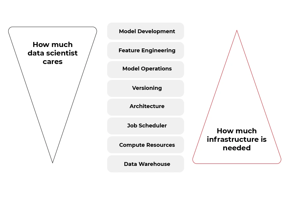
Fortunately, many of the tasks from the second bucket (infrastructure and software) can be automated. Some tools aim to boost the productivity of data scientists by allowing them to focus on the work of a data detective rather than on the productionization of solutions. And one of these tools is called Metaflow.
If you want to focus more on data science , less on engineering, but be able to scale every aspect of your work with no pain, you should take a look at how is Metaflow designed.
A Review of Metaflow
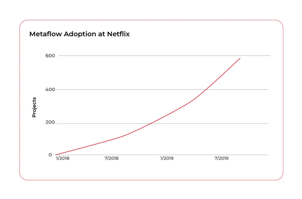
Metaflow is a framework for building and managing data science projects developed by Netflix. Before it was released as an open-source project in December 2019, they used it to boost the productivity of their data science teams working on a wide variety of projects from classical statistics to state-of-the-art deep learning.
The Metaflow library has Python and R API, however, almost 85% of the source code from the official repository (https://github.com/Netflix/metaflow) is written in Python. Also, separate documentation for R and Python is available.
At the time this article is written (July 2021), the official repository of the Metaflow has 4,5 k stars, above 380 forks, and 36 contributors, so it can be assumed as a mature framework.
“Metaflow is built for data scientists, not just for machines”
That sentence got attention when you visit the official website of the project ( https://metaflow.org/ ). Indeed, these are not empty words. Metaflow takes care of versioning, dependency management, computing resources, hyperparameters, parallelization, communication with AWS stack, and much more. You can truly focus on the core part of your data-related work and let Metaflow do all these things using just very expressive decorators.
Metaflow - core features
The list below explains the key features that make Metaflow such a wonderful tool for data scientists, especially for those who wish to remain ignorant in other areas.
- Abstraction over infrastructure. Metaflow provides a layer of abstraction over the hardware infrastructure available, cloud stack in particular. That’s why this tool is sometimes called a unified API to the infrastructure stack.
- Data pipeline organization. The framework represents the data flow as a directed acyclic graph. Each node in the graph, also called step, contains some code to run wrapped in a function with @step decorator.
@step
def get_lat_long_features(self):
self.features = coord_features(self.data, self.features)
self.next(self.add_categorical_features)
The nodes on each level of the graph can be computed in parallel, but the state of the graph between levels must be synchronized and stored somewhere (cached) – so we have very good asynchronous data pipeline architecture.

This approach facilitates debugging, enhances the performance of the pipeline, and allows us completely separate the steps so that we can run one step locally and the next one in the cloud if, for instance, the step requires solving large matrices. The disadvantage of that approach is that salient failures may happen without proper programming discipline.
- Versioning. Tracking versions of our machine learning models can be a challenging task. Metaflow can help here. The execution of each step of the graph (data, code, and parameters) is hashed and stored, and you can access logged data later, using client API.
- Containerization. Each step is run in a separate environment. We can specify conda libraries in each container using
@condadecorator as shown below. It can be a very useful feature under some circumstances.
@conda(libraries={"scikit-learn": "0.19.2"})
@step
def fit(self):
...
- Scalability. With the help of
@batchand@resourcesdecorators, we can simply command AWS Batch to spawn a container on ECS for the selected Metaflow step. If individual steps take long enough, the overhead of spawning the containers should become irrelevant.
@batch(cpu=1, memory=500)
@step
def hello(self):
...
- Hybrid runs. We can run one step locally and another compute-intensive step on the cloud and swap between these two modes very easily.
- Error handling. Metaflow’s
@retrydecorator can be used to set the number of retries if the step fails. Any error raised during execution can be handled by@catchdecorator. The@timeoutdecorator can be used to limit long-running jobs especially in expensive environments (for example with GPGPUs).
@catch(var="compute_failed")
@retry
@step
def statistics(self):
...
- Namespaces. An isolated production namespace helps to keep production results separate from experimental runs of the same project running concurrently. This feature is very useful in bigger projects where more people is involved in development and deployment processes.
from metaflow import Flow, namespace
namespace("user:will")
run = Flow("PredictionFlow").latest_run
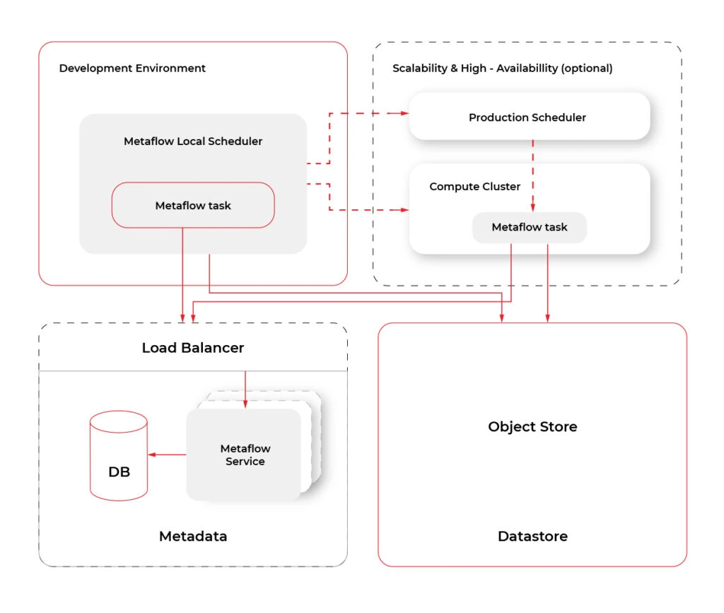
- Cloud Computing . Metaflow, by default, works in the local mode . However, the shared mode releases the true power of Metaflow. At the moment of writing, Metaflow is tightly and well coupled to AWS services like CloudFormation, EC2, S3, Batch, DynamoDB, Sagemaker, VPC Networking, Lamba, CloudWatch, Step Functions and more. There are plans to add more cloud providers in the future. The diagram below shows an overview of services used by Metaflow.
Metaflow - missing features
Metaflow does not solve all problems of data science projects. It’s a pity that there is only one cloud provider available, but maybe it will change in the future. Model serving in production could be also a really useful feature. Competitive tools like MLFlow or Apache AirFlow are more popular and better documented. Metaflow lacks a UI that would make metadata, logging, and tracking more accessible to developers. All this does not change the fact that Metaflow offers a unique and right approach, so just cannot be overlooked.
Conclusions
If you think Metaflow is just another tool for MLOps , you may be surprised. Metaflow offers data scientists a very comfortable workflow abstracting them from all low levels of that stuff. However, don't expect the current version of Metaflow to be perfect because Metaflow is young and still actively developed. However, the foundations are solid, and it has proven to be very successful at Netflix and outside of it many times.

Monitoring your microservices on AWS with Terraform and Grafana - basic microservices architecture
Do you have an application in the AWS cloud? Do you have several microservices you would like to monitor? Or maybe you’re starting your new project and looking for some good-looking, well-designed infrastructure? Look no further - you are in the right place!
We’ve spent some time building and managing microservices and cloud-native infrastructure so we provide you with a guide covering the main challenges and proven solutions.
In this series, we describe the following topics:
- How to create a well-designed architecture with microservices and a cloud-config server?
- How to collect metrics and logs in a common dashboard?
- How to secure the entire stack?
Monitoring your microservices - assumptions
Choosing Grafana for such a project seems obvious, as the tool is powerful, fast, user-friendly, customizable, and easy to maintain. Grafana works perfectly with Prometheus and Loki. Prometheus is a metric sink that collects metrics from multiple sources and sends them to the target monitoring system. Loki does the very same operation for logs. Both collectors are designed to be integrated with Grafana.
See the diagram below to better understand our architecture:
Let’s analyze the diagram for a moment. On the top, there is a publicly visible hosted zone in Route 53, the DNS “entry” to our system, with 3 records: two application services available over the internet and an additional monitoring service for our internal purposes.
Below, there is a main VPC with two subnets: public and private. In the public one, we have load balancers only, and in the private one, there is an ECS cluster. In the cluster, we have few services running using Fargate: two with internet-available APIs, two for internal purposes, one Spring Cloud Config Server, and our monitoring stack: Loki, Prometheus, and Grafana. At the bottom of the diagram, you can also find a Service Discovery service (AWS CloudMap) that creates entries in Route 53, to enable communication inside our private subnet.
Of course, for readability reasons, we omit VPC configuration, services dependencies (RDS, Dynamo, etc.), CI/CD, and all other services around the core. You can follow this guide covering building AWS infrastructure.
To sum up our assumptions:
- We use an infra-as-a-code approach with Terraform
- There are few Internet-facing services and few for internal purposes in our private subnet
- Internet-facing services are exposed via load balancers in the public subnet
- We use the Fargate launch type for ECS tasks
- Some services can be scaled with ECS auto-scaling groups
- We use Service Discovery to redeploy and scale without manual change of IP’s, URL’s or target groups
- We don’t want to repeat ourselves so we use a Spring Cloud Config Server as a main source of configuration
- We use Grafana to see synchronized metrics and logs
- (what you cannot see on the diagram) We use encrypted communication everywhere - including communication between services in a private subnet
Basic AWS resources
In this article, we assume you have all basic resources already created and correctly configured: VPC, subnets, general security groups, network ACLs, network interfaces, etc. Therefore we’re going to focus on resources visible on the diagram above, crucial from a monitoring point of view.
Let’s create the first common resource:
resource "aws_service_discovery_private_dns_namespace" "namespace_for_environment" {
name = "internal"
vpc = var.vpc_id
}
This is the Service Discovery visible in the lower part of the diagram. We’re going to fill it in a moment.
By the way, above, you can see an example, how we’re going to present listings. You will need to adjust some variables for your needs (like var .vpc_id ). We strongly recommend using Terragrunt to manage dependencies between your Terraform modules, but it’s out of the scope of this paper.
Your services without monitoring
Internet-facing services
Now let’s start with the first application. We need something to monitor.
resource "aws_route53_record" "foo_entrypoint" {
zone_id = var.zone_environment_id
name = "foo"
type = "A"
set_identifier = "foo.example.com"
alias {
name = aws_lb.foo_ecs_alb.dns_name
zone_id = aws_lb.foo_ecs_alb.zone_id
evaluate_target_health = true
}
latency_routing_policy {
region = var.default_region
}
}
This is an entry for Route53 to access the internet-facing “foo” service. We’ll use it to validate a TLS certificate later.
resource "aws_lb" "foo_ecs_alb" {
name = "foo"
internal = false
load_balancer_type = "application"
security_groups = [
aws_security_group.alb_sg.id
]
subnets = var.vpc_public_subnet_ids
}
resource "aws_lb_target_group" "foo_target_group" {
name = "foo"
port = 8080
protocol = "HTTP"
target_type = "ip"
vpc_id = var.vpc_id
health_check {
port = 8080
protocol = "HTTP"
path = "/actuator/health"
matcher = "200"
}
depends_on = [
aws_lb.foo_ecs_alb
]
}
resource "aws_lb_listener" "foo_http_listener" {
load_balancer_arn = aws_lb.foo_ecs_alb.arn
port = "8080"
protocol = "HTTP"
default_action {
type = "forward"
target_group_arn = aws_lb_target_group.foo_target_group.arn
}
}
resource "aws_security_group" "alb_sg" {
name = "alb-sg"
description = "Inet to ALB"
vpc_id = var.vpc_id
ingress {
protocol = "tcp"
from_port = 8080
to_port = 8080
cidr_blocks = [
"0.0.0.0/0"
]
}
egress {
protocol = "-1"
from_port = 0
to_port = 0
cidr_blocks = [
"0.0.0.0/0"
]
}
}
OK, what do we have so far?
Besides the R53 entry, we’ve just created a load balancer, accepting traffic on 8080 port and transferring it to the target group called foo_target_group . We use a default Spring Boot " /actuator/health " health check endpoint (you need to have spring-boot-starter-actuator dependency in your pom) and a security group allowing ingress traffic to reach the load balancer and all egress traffic from the load balancer.
Now, let’s create the service.
resource "aws_ecr_repository" "foo_repository" {
name = "foo"
}
resource "aws_ecs_task_definition" "foo_ecs_task_definition" {
family = "foo"
network_mode = "awsvpc"
requires_compatibilities = ["FARGATE"]
cpu = "512"
memory = "1024"
execution_role_arn = var.ecs_execution_role_arn
container_definitions = <<TASK_DEFINITION
[
{
"cpu": 512,
"image": "${aws_ecr_repository.foo_repository.repository_url}:latest",
"memory": 1024,
"memoryReservation" : 512,
"name": "foo",
"networkMode": "awsvpc",
"essential": true,
"environment" : [
{ "name" : "SPRING_CLOUD_CONFIG_SERVER_URL", "value" : "configserver.internal" },
{ "name" : "APPLICATION_NAME", "value" : "foo" }
],
"portMappings": [
{
"containerPort": 8080,
"hostPort": 8080
}
]
}
]
TASK_DEFINITION
}
resource "aws_ecs_service" "foo_service" {
name = "foo"
cluster = var.ecs_cluster_id
task_definition = aws_ecs_task_definition.foo_ecs_task_definition.arn
desired_count = 2
launch_type = "FARGATE"
network_configuration {
subnets = var.vpc_private_subnet_ids
security_groups = [
aws_security_group.foo_lb_to_ecs.id,
aws_security_group.ecs_ecr_security_group.id,
aws_security_group.private_security_group.id
]
}
service_registries {
registry_arn = aws_service_discovery_service.foo_discovery_service.arn
}
load_balancer {
target_group_arn = aws_lb_target_group.foo_target_group.arn
container_name = "foo"
container_port = 8080
}
depends_on = [aws_lb.foo_ecs_alb]
}
You can find just three resources above, but a lot of configuration. The first one is easy - just an ECR for the image of your application. Then we have a task definition. Please pay attention to environment variables SPRING_CLOUD_CONFIG_SERVER_URL - this is an address of our config server inside our internal Service Discovery domain. The third one is an ECS service.
As you can see, it uses some magic of ECS Fargate - automatically registering new tasks in a Service Discovery ( service_registries section) and a load balancer ( load_balancer section). We just need to wait until the load balancer is created ( depends_on = [aws_lb.foo_ecs_alb] ). If you want to add some autoscaling, this is the right place to put it in. You’re also ready to push your application to the ECR if you already have one. We’re going to cover the application's important content later in this article. The ecs_execution_role_arn is just a standard role with AmazonECSTaskExecutionRolePolicy , allowed to be assumed by ECS and ecs-tasks.
Let’s discuss security groups now.
resource "aws_security_group" "foo_lb_to_ecs" {
name = "allow_lb_inbound_foo"
description = "Allow inbound Load Balancer calls"
vpc_id = var.vpc_id
ingress {
from_port = 8080
protocol = "tcp"
to_port = 8080
security_groups = [aws_security_group.foo_alb_sg.id]
}
}
resource "aws_security_group" "ecs_to_ecr" {
name = "allow_ecr_outbound"
description = "Allow outbound traffic for ECS task, to ECR/docker hub"
vpc_id = aws_vpc.main.id
egress {
from_port = 443
to_port = 443
protocol = "tcp"
cidr_blocks = ["0.0.0.0/0"]
}
egress {
from_port = 53
to_port = 53
protocol = "udp"
cidr_blocks = ["0.0.0.0/0"]
}
egress {
from_port = 53
to_port = 53
protocol = "tcp"
cidr_blocks = ["0.0.0.0/0"]
}
}
resource "aws_security_group" "private_inbound" {
name = "allow_inbound_within_sg"
description = "Allow inbound traffic inside this SG"
vpc_id = var.vpc_id
ingress {
from_port = 0
to_port = 0
protocol = "-1"
self = true
}
egress {
from_port = 0
to_port = 0
protocol = "-1"
self = true
}
}
As you can see, we use three groups - all needed. The first one allows the load balancer located in the public subnet to call the task inside the private subnet. The second one allows our ECS task to poll its image from the ECR. The last one allows our services inside the private subnet to talk to each other - such communication is allowed by default, only if you don’t attach any specific group (like the load balancer’s one), therefore we need to explicitly permit this communication.
There is just one piece needed to finish the “foo” service infrastructure - the service discovery service entry.
resource "aws_service_discovery_service" "foo_discovery_service" {
name = "foo"
description = "Discovery service name for foo"
dns_config {
namespace_id = aws_service_discovery_private_dns_namespace.namespace_for_environment.id
dns_records {
ttl = 100
type = "A"
}
}
}
It creates a “foo” record in an “internal” zone. So little and yet so much. The important thing here is - this is a multivalue record, which means it can cover 1+ entries - it provides basic, equal-weight autoscaling during normal operation but Prometheus can dig out from such a record each IP address separately to monitor all instances.
Now some good news - you can simply copy-paste the code of all resources with names prefixed with “foo_” and create “bar_” clones for the second, internet-facing service in the project. This is what we love Terraform for.
Backend services (private subnet)
This part is almost the same as the previous one, but we can simplify some elements.
resource "aws_ecr_repository" "backend_1_repository" {
name = "backend_1"
}
resource "aws_ecs_task_definition" "backend_1_ecs_task_definition" {
family = "backend_1"
network_mode = "awsvpc"
requires_compatibilities = ["FARGATE"]
cpu = "512"
memory = "1024"
execution_role_arn = var.ecs_execution_role_arn
container_definitions = <<TASK_DEFINITION
[
{
"cpu": 512,
"image": "${aws_ecr_repository.backend_1_repository.repository_url}:latest",
"memory": 1024,
"memoryReservation" : 512,
"name": "backend_1",
"networkMode": "awsvpc",
"essential": true,
"environment" : [
{ "name" : "_JAVA_OPTIONS", "value" : "-Xmx1024m -Xms512m" },
{ "name" : "SPRING_CLOUD_CONFIG_SERVER_URL", "value" : "configserver.internal" },
{ "name" : "APPLICATION_NAME", "value" : "backend_1" }
],
"portMappings": [
{
"containerPort": 8080,
"hostPort": 8080
}
]
}
]
TASK_DEFINITION
}
resource "aws_ecs_service" "backend_1_service" {
name = "backend_1"
cluster = var.ecs_cluster_id
task_definition = aws_ecs_task_definition.backend_1_ecs_task_definition.arn
desired_count = 1
launch_type = "FARGATE"
network_configuration {
subnets = var.vpc_private_subnet_ids
security_groups = [
aws_security_group.ecs_ecr_security_group.id,
aws_security_group.private_security_group.id
]
}
service_registries {
registry_arn = aws_service_discovery_service.backend_1_discovery_service.arn
}
}
resource "aws_service_discovery_service" "backend_1_discovery_service" {
name = "backend1"
description = "Discovery service name for backend 1"
dns_config {
namespace_id = aws_service_discovery_private_dns_namespace.namespace_for_environment.id
dns_records {
ttl = 100
type = "A"
}
}
}
As you can see, all resources related to the load balancer are gone. Now, you can copy the code about creating the backend_2 service.
So far, so good. We have created 4 services, but none will start without the config server yet.
Config server
The infrastructure for the config server is similar to the backed services described above. It simply needs to know all other services’ URLs. In the real-world scenario, the configuration may be stored in a git repository or in the DB, but it’s not needed for this article, so we’ve used a native config provider, with all config files stored locally.
We would like to dive into some code here, but there is not much in this module yet. To make it just working, we only need this piece of code:
@SpringBootApplication
@EnableConfigServer
public class CloudConfigServer {
public static void main(String[] arguments) {
run(CloudConfigServer.class, arguments);
}
}
and few dependencies.
<dependency>
<groupId>org.springframework.cloud</groupId>
<artifactId>spring-cloud-config-server</artifactId>
</dependency>
<dependency>
<groupId>org.springframework.boot</groupId>
<artifactId>spring-boot-starter-security</artifactId>
</dependency>
<dependency>
<groupId>org.springframework.boot</groupId>
<artifactId>spring-boot-starter-web</artifactId>
</dependency>
We also need some extra config in the pom.xml file.
<parent>
<groupId>org.springframework.boot</groupId>
<artifactId>spring-boot-starter-parent</artifactId>
<version>2.4.2</version>
</parent>
<dependencyManagement>
<dependencies>
<dependency>
<groupId>org.springframework.cloud</groupId>
<artifactId>spring-cloud-dependencies</artifactId>
<version>2020.0.1</version>
<type>pom</type>
<scope>import</scope>
</dependency>
</dependencies>
</dependencyManagement>
<build>
<plugins>
<plugin>
<groupId>org.springframework.boot</groupId>
<artifactId>spring-boot-maven-plugin</artifactId>
</plugin>
</plugins>
</build>
That’s basically it - you have your own config server. Now, let’s put some config inside. The Structure of the server is as follows.
config_server/
├─ src/
│ ├─ main/
│ ├─ java/
│ ├─ com/
│ ├─ example/
│ ├─ CloudConfigServer.java
│ ├─ resources/
│ ├─ application.yml (1)
│ ├─ configforclients/
│ ├─ application.yml (2)
As there are two files called application.yml we’ve added numbers (1), (2) at the end of lines to distinguish them. So the application.yml (1) file is there to configure the config server itself. Its content is as follows:
server:
port: 8888
spring:
application:
name: spring-cloud-config-server
profiles:
include: native
cloud:
config:
server:
native:
searchLocations: classpath:/configforclients
management:
endpoints:
web:
exposure:
include: health
With the “native” configuration, the entire classpath:/ and classpath:/config are taken as a configuration for remote clients. Therefore, we need this line:
spring.cloud.config.server.native.searchLocations: classpath:/configforclients to distinguish the configuration for the config server itself and for the clients. The client’s configuration is as follows:
address:
foo: ${FOO_URL:http://localhost:8080}
bar: ${BAR_URL:http://localhost:8081}
backend:
one: ${BACKEND_1_URL:http://localhost:8082}
two: ${BACKEND_2_URL:http://localhost:8083}
management:
endpoints:
web:
exposure:
include:health
spring:
jackson:
default-property-inclusion: non_empty
time-zone: Europe/Berlin
As you can see, all service discovery addresses are here, so they can be used by all clients. We also have some common configurations, like Jackson-related, and one important for the infra - to expose health checks for load balancers.
If you use Spring Boot Security (I hope you do), you can disable it here - it will make accessing the config server simpler, and, as it’s located in the private network and we’re going to encrypt all endpoints in a moment - you don’t need it. Here is an additional file to disable it.
@Configuration
@EnableWebSecurity
public class WebSecurityConfig extends WebSecurityConfigurerAdapter {
@Override
public void configure(WebSecurity web) throws Exception {
web.ignoring().antMatchers("/**");
getHttp().csrf().disable();
}
}
Yes, we know, it's strange to use @EnableWebSecurity to disable web security, but it’s how it works. Now, let’s configure clients to read those configurations.
Config clients
First of all, we need two dependencies.
<dependency>
<groupId>org.springframework.cloud</groupId>
<artifactId>spring-cloud-starter-bootstrap</artifactId>
</dependency>
<dependency>
<groupId>org.springframework.cloud</groupId>
<artifactId>spring-cloud-starter-config</artifactId>
</dependency>
We assume you have all Spring-Boot related dependencies already in place.
As you can see, we need to use bootstrap, so instead of the application.yml file, we’re going to use bootstrap.yml(which is responsible for loading configuration from external sources):
main:
banner-mode: 'off'
cloud:
config:
uri: ${SPRING_CLOUD_CONFIG_SERVER:http://localhost:8888}
There are only two elements here. We use the first one just to show you that some parameters simply cannot be set using the config server. In this example, main.banner-mode is being read before accessing the config server, so if you want to disable the banner (or change it) - you need to do it in each application separately. The second property - cloud.config.uri - is obviously a pointer to the config server. As you can see, we use a fallback value to be able to run everything both in AWS and local machines.
Now, with this configuration, you can really start every service and make sure that everything works as expected.
Monitoring your microservices - conclusion
That was the easy part. Now you have a working application, exposed and configurable. We hope you can tweak and adjust it for your own needs. In the next part we’ll dive into a monitoring topic.

How to achieve sustainable mobility using sustainable software development
Should the code be green?
Sustainable Mobility is the key goal for today and future vehicle manufacturers and mobility providers. Reducing the CO2 footprint of transportation contributes to building a better future for all of us. For the automotive industry, part of this goal is defined in the European Vehicle Emission Standards initiative, Euro 7 being the latest norm before all cars become fully zero-emission.
There are multiple paths leading into zero-emission transportation, most of which are being taken in parallel. Electric vehicles, especially charged using renewable energy sources such as solar energy. Fuel cells and hydrogen vehicles. Using recycled materials for both car interior and exterior. Car sharing, better urban transportation, and all kinds of initiatives leading to reducing the number of vehicles on the roads.
How software development companies can help us achieve sustainable mobility
Of course, software development companies can help with these kinds of initiatives by building software platforms for electric vehicles , efficient charging, and navigating to charging stations using renewable energy or making sure supply chains are fully invested in reducing CO2 emissions.
But is there anything, in general, we can do, or at least think about, to make software development more environment-aware?
One important aspect is the computational complexity of the code. More operations, assuming the same hardware, require more energy. This is especially important these days, as the microprocessors availability has become a huge bottleneck for the automotive industry. How can we mitigate this problem? Let’s look at two possibilities.
Building software for sustainable mobility with green coding
Firstly, does the programming language or code quality matter? Yes and yes. Let’s start by looking at the Energy Efficiency across Programming Languages paper from 2017 comparing the energy efficiency of programming languages (the lower, the better):
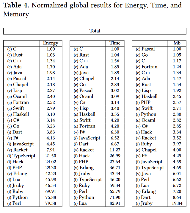
We can see that switching to a lower-level language can improve energy consumption. Is this the answer to the problem? Not directly. Procedural, statically typed languages are, in general, faster and have lower energy consumption, but at the same time are more complicated and require more time to write the same amount of code in easier to use ones. This is not a hard rule, as we can see Java gets a great result, although probably after optimizations.
Choosing energy-efficient computing resources
So one thing we can do is to think about the efficiency of the language when we choose the tech stack for our project. The other thing regarding the same problem is to optimize the code instead of adding more cores or GBs of memory - as it may be a cheaper solution initially.
The other improvement we can make comes to leveraging shared resources in the cloud for computation by building multi-layer computing systems, where results required immediately or in real-time can be computed on edge devices, while others can be computed at the edge of the cloud or in distributed cloud systems. Having those three layers, where two of them share resources between multiple vehicles or end-user devices, makes the computation both more cost-effective and requires less energy, as the bill is shared between multiple users.
Developers and software development departments can contribute to making the sustainable mobility goal achievable in the near future. Small steps and decisions regarding programming languages, frameworks, computing resources make a difference.
Serverless architecture with AWS Cloud Development Kit (CDK)
The IT world revolves around servers - we set up, manage, and scale them, we communicate with them, deploy software onto them, and restrict access to them. In the end, it is difficult to imagine our lives without them. However, in this “serverfull” world, an idea of serverless architecture arose. A relatively new approach to building applications without direct access to the servers required to run them. Does it mean that the servers are obsolete, and that we no longer should use them? In this article, we will explore what it means to build a serverless application, how it compares to the well-known microservice design, what are the pros and cons of this new method and how to use the AWS Cloud Development Kit framework to achieve that.
Background
There was a time when the world was inhabited by creatures known as “monolith applications”. Those beings were enormous, tightly coupled, difficult to manage, and highly resource-consuming, which made the life of tech people a nightmare.
Out of that nightmare, a microservice architecture era arose, which was like a new day for software development. Microservices are small independent processes communicating with each other through their APIs. Each microservice can be developed in a different programming language, best suited for its job, providing a great deal of flexibility for developers. Although the distributed nature of microservices increased the overall architectural complexity of the systems, it also provided the biggest benefit of the new approach, namely scalability, coming from the possibility to scale each microservice individually based on its resource demands.
The microservice era was a life changer for the IT industry. Developers could focus on the design and development of small modular components instead of struggling with enormous black box monoliths. Managers enjoyed improvements in efficiency. However, microservice architecture still posed a huge challenge in the areas of deployment and infrastructure management for distributed systems. What is more, there were scenarios when it was not as cost-effective as it could be. That is how the software architecture underwent another major shift. This time towards the serverless architecture epoch.
What is serverless architecture?
Serverless, a bit paradoxically, does not mean that there are no servers. Both server hardware and server processes are present, exactly as in any other software architecture. The difference is that the organization running a serverless application is not owning and managing those servers. Instead, they make use of third-party Backend as a Service (BaaS) and/or Function as a Service platform.
- Backend as a Service (BaaS) is a cloud service model where the delivery of services responsible for server-side logic is delegated to cloud providers. This often includes services such as: database management, cloud storage, user authentication, push notifications, hosting, etc. In this approach, client applications, instead of talking to their dedicated servers, directly operate on those cloud services.

- Function as a Service (FaaS) is a way of executing our code in stateless, ephemeral computing environments fully managed by third-party providers without thinking about the underlying servers. We simply upload our code, and the FaaS platform is responsible for running it. Our functions can then be triggered by events such as HTTP(S) requests, schedulers, or calls from other cloud services. One of the most popular implementations of FaaS is the AWS Lambda service, but each cloud provider has its corresponding options.

In this article, we will explore the combination of both BaaS and FaaS approaches as most enterprise-level solutions combine both of them into a fully functioning system.
Note: This article is often referencing services provided by AWS . However, it is important to note that the serverless architecture approach is not cloud-provider-specific and most of the services mentioned as part of the AWS platform have their equivalents in other cloud platforms.
Serverless architecture design
We know a bit of theory, so let us look now at a practical example. The figure 1 presents an architecture diagram of a user management system created with the serverless approach.

The system utilizes Amazon Cognito for user authentication and authorization, ensuring that only authorized parties access our API. Then we have the API Gateway, which deals with all the routing, requests throttling, DDOS protection etc. API Gateway also allows us to implement custom authorizers if we can’t or don’t want to use Amazon Cognito. The business logic layer consists of Lambda Functions. If you are used to the microservice approach, you can think of each lambda as a separate set of a controller endpoint and service method, handling a specific type of request. Lambdas further communicate with other services such as databases, caches, config servers, queues, notification services, or whatever else our application may require.
The presented diagram demonstrates a relatively simple API design. However, it is good to bear in mind that the serverless approach is not limited to APIs. It is also perfect for more complex solutions such as data processing, batch processing, event ingestion systems, etc.
Serverless vs Microservices
Microservice-oriented architecture broke down the long-lasting realm of monolith systems through the division of applications into small, loosely coupled services that could be developed, deployed, and maintained independently. Those services had distinct responsibilities and could communicate with each other through APIs, constituting together a much larger and complex system. Up till this point, serverless does not differ much from the microservice approach. It also divides a system into smaller, independent components, but instead of services, we usually talk about functions.
So, what’s the difference? The microservices are standalone applications, usually packaged as lightweight containers and run on physical servers (commonly in the cloud), which you can access, manage and scale if needed. Those containers need to be supervised (orchestrated) with the use of tools such as Kubernetes . So speaking simply, you divide your application into smaller independent parts, package them as containers, deploy on servers, and orchestrate their lifecycle.
In comparison, when it comes to serverless functions, you only write your function code, upload it to the FaaS provider platform, and the cloud provider handles its packaging, deployment, execution, and scaling without showing you (or giving you access to) physical resources required to run it. What is more, when you deploy microservices, they are always active, even when they do not perform any processing, on the servers provisioned to them. Therefore, you need to pay for required host servers on a daily or monthly basis, in contrast to the serverless functions, which are only brought to life for their time of execution, so if there are no requests they do not use any resources.

Pros & cons of serverless computing
Pros:
- Pricing - Serverless works in a pay-as-you-go manner, which means that you only pay for those resources which you actually use, with no payment for idle time of the servers and no in-front dedication. This is especially beneficial for applications with infrequent traffic or startup organizations.
- Operational costs and complexity - The management of your infrastructure is delegated almost entirely to the cloud provider. This frees up your team allocation, decreases the probability of error on your side, and automates downtime handling leading to the overall increase in the availability of your system and the decrease in operational costs.
- Scalability by design - Serverless applications are scalable by nature. The cloud provider handles scaling up and down of resources automatically based on the traffic.
Cons:
- It is a much less mature approach than microservices which means a lot of unknowns and spaces for bad design decisions exist.
- Architectural complexity - Serverless functions are much more granular than microservices, and that can lead to higher architectural complexity, where instead of managing a dozen of microservices, you need to handle hundreds of lambda functions.
- Cloud provider specific solutions - With microservices packaged as containers, it didn’t matter which cloud provider you used. That is not the case for serverless applications which are tightly bound to the services provided by the cloud platform.
- Services limitations - some Faas and BaaS services have limitations such as a maximum number of concurrent requests, memory, timeouts, etc. which are often customizable but only to a certain point (e.g., default AWS Lambda execution quota equals 1000).
- Cold starts - Serverless applications can introduce response delays when a new instance handles its first request because it needs to boot up, copy application code, etc. before it can run the logic.
How much does it really cost?
One of the main advantages of the serverless design is its pay-as-you-go model, which can greatly decrease the overall costs of your system. However, does it always lead to lesser expenses? For this consideration, let us look at the pricing of some of the most common AWS services.
Service Price API Gateway 3.50$ per 1M requests (REST Api) Lambda 0.20$ per 1M request SQS First 1M free, then 0.40& per 1M requests
Those prices seem low, and in many cases, they will lead to very cheap operational costs of running serverless applications. Having that said, there are some scenarios where serverless can get much more expensive than other architectures. Let us consider a system that handles 5 mln requests per hour. Having it designed as a serverless architecture will lead to the cost of API Gateway only equal to:
$3.50 * 5 * 24 * 30 = $12,600/month
In this scenario, it could be more efficient to have an hourly rate-priced load balancer and a couple of virtual machines running. Then again, we would have to take into consideration the operational cost of setting up and managing the load balancer and VMs. As you can see, it all depends on the specific use case and your organization. You can read more about this scenario in this article .
AWS Cloud Development Kit
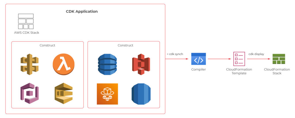
At this point, we know quite a lot about serverless computing, so now, let’s take a look at how we can create our serverless applications. First of all, we can always do it manually through the cloud provider’s console or CLI. It may be a valuable educational experience, but we wouldn’t recommend it for real-life systems. Another well-known solution is using Infrastructure as a Code (IaaS), such as AWS Cloud Formation service . However, in 2019 AWS introduced another possibility which is AWS Cloud Development Kit (CDK).
AWS CDK is an open-source software development framework which lets you define your architectures using traditional programming languages such as Java, Python, Javascript, Typescript, and C#. It provides you with high-level pre-configured components called constructs which you can use and further extend in order to build your infrastructures faster than ever. AWS CDK utilizes Cloud Formation behind the scenes to provision your resources in a safe and repeatable manner.
We will now take a look at the CDK definitions of a couple of components from the user management system, which the architecture diagram was presented before.
Main stack definition
export class UserManagerServerlessStack extends cdk.Stack {
private static readonly API_ID = 'UserManagerApi';
constructor(scope: cdk.Construct, id: string, props?: cdk.StackProps) {
super(scope, id, props);
const cognitoConstruct = new CognitoConstruct(this)
const usersDynamoDbTable = new UsersDynamoDbTable(this);
const lambdaConstruct = new LambdaConstruct(this, usersDynamoDbTable);
new ApiGatewayConstruct(this, cognitoConstruct.userPoolArn, lambdaConstruct);
}
}
API gateway
export class ApiGatewayConstruct extends Construct {
public static readonly ID = 'UserManagerApiGateway';
constructor(scope: Construct, cognitoUserPoolArn: string, lambdas: LambdaConstruct) {
super(scope, ApiGatewayConstruct.ID);
const api = new RestApi(this, ApiGatewayConstruct.ID, {
restApiName: 'User Manager API'
})
const authorizer = new CfnAuthorizer(this, 'cfnAuth', {
restApiId: api.restApiId,
name: 'UserManagerApiAuthorizer',
type: 'COGNITO_USER_POOLS',
identitySource: 'method.request.header.Authorization',
providerArns: [cognitoUserPoolArn],
})
const authorizationParams = {
authorizationType: AuthorizationType.COGNITO,
authorizer: {
authorizerId: authorizer.ref
},
authorizationScopes: [`${CognitoConstruct.USER_POOL_RESOURCE_SERVER_ID}/user-manager-client`]
};
const usersResource = api.root.addResource('users');
usersResource.addMethod('POST', new LambdaIntegration(lambdas.createUserLambda), authorizationParams);
usersResource.addMethod('GET', new LambdaIntegration(lambdas.getUsersLambda), authorizationParams);
const userResource = usersResource.addResource('{userId}');
userResource.addMethod('GET', new LambdaIntegration(lambdas.getUserByIdLambda), authorizationParams);
userResource.addMethod('POST', new LambdaIntegration(lambdas.updateUserLambda), authorizationParams);
userResource.addMethod('DELETE', new LambdaIntegration(lambdas.deleteUserLambda), authorizationParams);
}
}
CreateUser Lambda
export class CreateUserLambda extends Function {
public static readonly ID = 'CreateUserLambda';
constructor(scope: Construct, usersTableName: string, layer: LayerVersion) {
super(scope, CreateUserLambda.ID, {
...defaultFunctionProps,
code: Code.fromAsset(resolve(__dirname, `../../lambdas`)),
handler: 'handlers/CreateUserHandler.handler',
layers: [layer],
role: new Role(scope, `${CreateUserLambda.ID}_role`, {
assumedBy: new ServicePrincipal('lambda.amazonaws.com'),
managedPolicies: [
ManagedPolicy.fromAwsManagedPolicyName('service-role/AWSLambdaBasicExecutionRole'),
]
}),
environment: {
USERS_TABLE: usersTableName
}
});
}
}
User DynamoDB table
export class UsersDynamoDbTable extends Table {
public static readonly TABLE_ID = 'Users';
public static readonly PARTITION_KEY = 'id';
constructor(scope: Construct) {
super(scope, UsersDynamoDbTable.TABLE_ID, {
tableName: `${Aws.STACK_NAME}-Users`,
partitionKey: {
name: UsersDynamoDbTable.PARTITION_KEY,
type: AttributeType.STRING
} as Attribute,
removalPolicy: RemovalPolicy.DESTROY,
});
}
}
The code with a complete serverless application can be found on github: https://github.com/mkapiczy/user-manager-serverless
All in all, serverless architecture is becoming an increasingly attractive solution when it comes to the design of IT systems. Knowing what it is all about, how it works, and what are its benefits and drawbacks will help you make good decisions on when to stick to the beloved microservices and when to go serverless in order to help your organization grow .

Building intelligent document processing systems – entity finders
Our journey towards building Intelligent Document Processing systems will be completed with entity finders, components responsible for extracting key information.
This is the third part of the series about Intelligent Document Processing (IDP). The series consists of 3 parts:
- Problem definition and data
- Classification and validation
- Entity finders
Entity finders
After classifying the documents, we focus on extracting some class-specific information. We pose the main interests in the jurisdiction, property address, and party names. We called the components responsible for their extraction simply “finders”.
Jurisdictions showed they could be identified based on dictionaries and simple rules. The same applies to file dates.
Context finders
The next 3 entities – addresses, parties, and document dates, provide us with a challenge.
Let us note the fact that:
- Considering addresses. There may be as many as 6 addresses on a first page on its own. Some belong to document parties, some to the law office, others to other entities engaged in a given process. Somewhere in this maze of addresses, there is this one that we are interested in – property address. Or there isn’t - not every document has to have the address at all. Some have, often, only the pointers to the page or another document (which we need to extract as well).
- The case with document dates is a little bit simpler. Obviously, there are often a few dates in the document not mentioning any numbers, dates are in every format possible, but generally, the document date occurs and is possible to distinguish.
- Party names – arguably the hardest entities to find. Depending on the document, there may be one or more parties engaged or none. The difficulty is that virtually any name that represents a person, company, or institution in the document is a potential candidate for the party. The variability of contexts indicating that a given name represents a party is huge, including layout and textual contexts.
Generally, our solutions are based on three mechanisms.
- Context finders: We search for the contexts in which the searched entities may occur.
- Entity finders: We are estimating the probability that a given string is the search value.
- Managers: we merge the information about the context with the information About the values and decide whether the value is accepted
Address finder
Addresses are sometimes multi-line objects such as:
“LOT 123 OF THIS AND THIS ESTATES, A SUBDIVISION OF PART OF THE SOUTH HALF OF THE NORTHEAST QUARTER AND THE NORTH HALF OF THE SOUTHEAST QUARTER OF SECTION 123 (...)”.
It is possible that the address is written over more than one or a few lines. When such expression occurs, we are looking for something simpler like :
“The Institution, P.O. Box 123 Cheyenne, CO 123123”
But we are prepared for each type of address.
In the case of addresses, our system is classifying every line in a document as a possible address line. The classification is based on n-grams and other features such as the number of capital letters, the proportion of digits, proportion of special signs in a line. We estimate the probability of the address occurring in the line. Then we merge lines into possible address blocks.
The resulting blocks may be found in many places. Some blocks are continuous, but some pose gaps when a single line in the address is not regarded as probable enough. Similarly, there may occur a single outlier line. That’s why we smooth the probabilities with rules.
After we construct possible address blocks, we filter them with contexts.
We manually collected contexts in which addresses may occur. We can find them in the text later in a dictionary-like manner. Because contexts may be very similar but not identical, we can use Dynamic Time Warping.
An example of similar but not identical context may be:
“real property described as follows:”
“real property described as follow:”
Document date finder
Document dates are the easiest entities to find thanks to a limited number of well-defined contexts, such as “dated this” or “this document is made on”. We used frequent pattern mining algorithms to reveal the most frequent document date context patterns among training documents. After that, we marked every date occurrence in a given document using a modified open-source library from the python ecosystem. Then we applied context-based rules for each of them to select the most likely date as document date. This solution has an accuracy of 82-98% depending on the test set and labels quality.

Parties finder
It’s worth mentioning that this part of our solution together with the document dates finder is implemented and developed in the Julia language . Julia is a great tool for development on the edge of science and you can read about views on it in another blog post here.
The solution on its own is somehow similar to the previously described, especially to the document date finder. We omit the line classifier and emphasize the impact of the context. Here we used a very generic name finder based on regular expression and many groups of hierarchical contexts to mark potential parties and pick the most promising one.
Summary
This part concludes our project focused on delivering an Intelligent Document Processing system. As we also, AI enables us to automate and improve operations in various areas.
The processes in banks are often labor bound, meaning they can only take on as much work as the labor force can handle as most processes are manual and labor-intensive. Using ML to identify, classify, sort, file, and distribute documents would be huge cost savings and add scalability to lucrative value streams where none exists today.
Train your computer with the Julia programming language – Machine Learning in Julia
Once we know the basics of Julia , we focus on its utilization in building machine learning software. We go through the most helpful tools and moving from prototyping to production.
How to do Machine Learning in Julia
Machine Learning tools dedicated to Julia have evolved very fast in the last few years. In fact, quite recently, we can say that Julia is production-ready! - as it was announced on JuliaCon2020.
Now, let's talk about the native tools available in Julia's ecosystem for Data Scientists. Many libraries and frameworks that serve machine learning models are available in Julia. In this article, we focus on a few the most promising libraries.
Da t aFrames.jl is a response to the great popularity of pandas – a library for data analysis and manipulation, especially useful for tabular data. DataFrames module plays a central role in the Julia data ecosystem and has tight integrations with a range of different libraries. DataFrames are essentially collections of aligned Julia vectors so they can be easily converted to other types of data like Matrix. Pand as.jl package provides binding to the pandas' library if someone can’t live without it, but we recommend using a native DataFrames library for tabular data manipulation and visualization.
In Julia, usually, we don’t need to use external libraries as we do with numpy in Python to achieve a satisfying performance of linear algebra operations. Native Arrays and Matrices may perform satisfactorily in many cases. Still, if someone needs more power here there is a great library StaticArrays.jl implementing statically sized arrays in Julia. Potential speedup falls in a range from 1.8x to 112.9x if the array isn’t big (based on tests provided by the authors of the library).
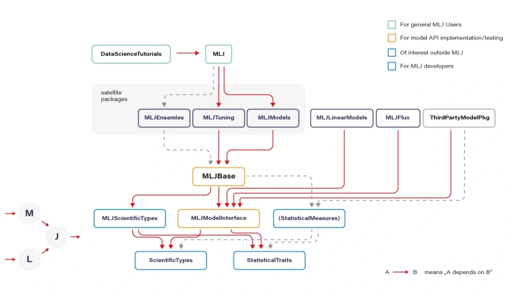
MLJ.jl created by Alan Turing Institute provides a common interface and meta-algorithms for selecting, tuning, evaluating, composing, and comparing over 150 machine learning models written in Julia and other languages. The library offers an API that lets you manage ML workflows in many aspects. Some parts of the API syntax may seem unfamiliar to the audience but remains clear and easy to use.
Flux.jl defines models just like mathematical notation. Provides lightweight abstractions on top of Julia's native GPU and TPU - GPU kernels can be written directly in Julia via CU DA.jl. Flux has its own Model Zoo and great integration with Julia’s ecosystem.
MXNet.jl is a part of a big Apache MXNet project. MXNet brings flexible and efficient GPU computing and state-of-art deep learning to Julia. The library offers very efficient tensor and matrix computation across multiple CPUs, GPUs, and disturbed server nodes.
Knet.jl (pronounced "kay-net") is the Koç University deep learning framework. The library supports GPU operations and automates differentiation using dynamic computational graphs for models defined in plain Julia.
AutoMLPipeline is a package that makes it trivial to create complex ML pipeline structures using simple expressions. AMLP leverages on the built-in macro programming features of Julia to symbolically process, manipulate pipeline expressions, and makes it easy to discover optimal structures for machine learning prediction and classification.
There are many more specific libraries like DecisionTree.jl , Transformers.jl, or YOLO.jl which are often immature but still can be utilized. Obviously, bindings to other popular ML frameworks exists, where many people may find TensorFlow.jl , Torch.jl, or ScikitLearn.jl as useful. We recommend using Flux or MLJ as the default choice for a new ML project.
Now let’s discuss the situation when Julia is not ready. And here, PyCall.jl comes to the rescue. The Python ecosystem is far greater than Julia’s. Someone could argue here that using such a connector loses all of the speed gained from using Julia and can even be slower than using Python standalone. Well, that’s true. But it’s worth to realize that we ask PyCall for help not so often because the number of native Julia ML libraries is quite good and still growing. And even if we ask, the scope is usually limited to narrow parts of our algorithms.
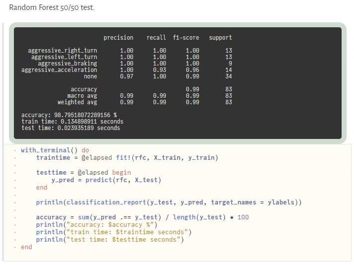
Sometimes sacrificing a part of application performance can be a better choice than sacrificing too much of our time, especially during prototyping. In a production environment, the better idea may be (but it's not a rule) to call to a C or C++ API of some of the mature ML frameworks (there are many of them) if a Julia equivalent is not available. Here is an example of how easily one can use the famous python scikit-learn library during prototyping:
@sk_import ensemble: RandomForestClassifier; fit!(RandomForestClassifier(), X, y)
The powerful metaprogramming features ( @sk_import macro via PyCall) take care of everything, exposing clean and functional style API of the selected package. On the other hand, because the Python ecosystem is very easily accessible from Julia (thanks to PyCall), many packages depend on it, and in turn, depend on Python, but that’s another story.
From prototype to Pproduction
In this section, we present a set of basic tools used in a typical ML workflow, such as writing a notebook, drawing a plot, deploying an ML model to a webserver or more sophisticated computing environments. I want to emphasize that we can use the same language and the same basic toolset for every stage of the machine learning software development process: from prototyping to production at full speed.
For writing notebooks, there are two main libraries available. IJulia.jl is a Jupyter language kernel and works with a variety of notebook user interfaces. In addition to the classic Jupyter Notebook, IJulia also works with JupyterLab, a Jupyter-based integrated development environment for notebooks and code. This option is more conservative.
For anyone who’s looking for something fresh and better, there is a great project called Pluto.jl - a reactive, lightweight and simple notebook with beautiful UI. Unlike Jupyter or Matlab, there is no mutable workspace, but an important guarantee: At any instant, the program state is completely described by the code you see. No hidden state, no hidden bugs. Changing one cell instantly shows effects on all other cells thanks to the reactive technologies used. And the most important feature: your notebooks are saved as pure Julia files! You can also export your notebook as HTML and PDF documents.
Visualization and plotting are essential parts of a typical machine learning workflow. We have several options here. For tabular data visualization there we can just simply use the DataFrame variable in a printable context. In Pluto, it looks really nice (and is interactive):
The primary option for plotting is Plots.jl , a plotting meta package that brings many different plotting packages under a single API, making it easy to swap between plotting "backends". This is a mature package with a large number of features (including 3D plots). The downside is that it uses Python behind the scenes (but that’s not a severe issue here) and can cause problems with configuration.
Gadfly.jl is based largely on ggplot2 for R and renders high-quality graphics to SVG, PNG, Postscript, and PDF. The interface is simple and cooperates well with DataFrames.
There is an interesting package called StatsPlots.jl which is a replacement for Plots.jl that contains many statistical recipes for concepts and types introduced in the JuliaStats organization, including correlation plot, Andrew's plot, MDS plot, and many more.
To expose the ML model as a service, we can establish a custom model server. To do so, we can use Genie.jl - a full-stack MVC web framework that provides a streamlined and efficient workflow for developing modern web applications and much more. Genie manages all of the virtual environments, database connectivity, or automatic deployment into docker containers (you just run one function, and everything works). It’s pure Julia and that’s important here because this framework manages the entire project for you. And it’s really very easy to use.
Apache Spark is a distributed data and computation engine that becomes more and more popular, especially among large companies and corporations. Hosted Spark instances offered by cloud service providers make it easy to get started and to run large, on-demand clusters for dynamic workloads.
While Scala, as the primary language of Spark, is not the best choice for some numerical computing tasks, being built for numerical computing, Julia is however perfectly suited to create fast and accurate numerical applications. Spark.jl is a library for that purpose. It allows you to connect to a Spark cluster from the Julia REPL and load data and submit jobs. It uses JavaCall.jl behind the scenes. This package is still in the initial development phase. Someone said that Julia is a bridge between Python and Spark - being simple like Python but having the big-data manipulation capabilities of Spark.
In Julia, we can do distributed computing effortlessly. We can do it with a useful JuliaDB.jl package, but straight Julia with distributed processes work well. We use it in production, distributed across multiple servers at scale. Implementation of distributed parallel computing is provided by module Distributed as part of the standard library shipped with Julia.
Machine Learning in Julia - conclusions
We covered a lot of topics, but in fact, we only scratched the surface. Presented examples show that, under certain conditions, Julia can be considered as a serious option for your next machine learning project in an enterprise environment or scientific work. Some Rustaceans (Rust language users call themselves that) ask themselves in terms of machine learning capabilities in their loved language: Are we learning yet? Julia's users can certainly answer yes! Are we production ready? Yes, but it doesn't mean Julia is the best option for your machine learning projects. More often, the mature Python ecosystem will be the better choice. Is Julia the future of machine learning? We believe so, and we’re looking forward to see some interesting apps written with Julia.
Building intelligent document processing systems - classification and validation
We continue our journey towards building Intelligent Document Processing Systems. In this article, we focus on document classification and validation.
This is the second part of the series about Intelligent Document Processing ( IDP ). The series consists of 3 parts:
- Problem definition and data
- Classification and validation
- Entities finders
If you are interested in data preparation, read the previous article. We describe there what we have done to get the data transformed into the form.
Classes
The detailed classification of document types shows that documents fall into around 80 types. Not every type is well-represented, and some of them have a minor impact or neglectable specifics that would force us to treat them as a distinct class.
After understanding the specifics, we ended up with 20 classes of documents. Some classes are more general, such as Assignment, some are as specific as Bankruptcy. The types we classify are: Assignment, Bill, Deed, Deed Of Separation, Deed Of Subordination, Deed Of Trust, Foreclosure, Deed In Lieu Foreclosure, Lien, Mortgage, Trustees Deed, Bankruptcy, Correction Deed, Lease, Modification, Quit Claim Deed, Release, Renunciation, Termination.
We chose these document types after summarizing the information present in each type. When the following services and routing are the same for similar documents, we do not distinguish them in target classes. We abandoned a few other types that do not occur in the real world often.
Classification
Our objective was to classify them for the correct next routing and for the application of the consecutive services. For example, when we are looking for party names, dealing with the Bankruptcy type of document, we are not looking for more than one legal entity.
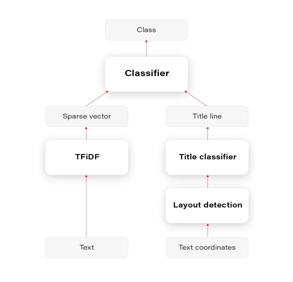
The documents are long and various. We can now start to think about the mathematical representation of them. Neural networks can be viewed as a complex encoders with classifier on top. These encoders are usually, in fact, powerful systems that can comprehend a lot of content and dependencies in text. However, the longer the text, the harder for a network to focus on a single word or single paragraph. There was a lot of research that confirms our intuition, which shows that the responsibility of classification of long documents on huge encoders is on the final layer and embeddings could be random to give similar results.
Recent GPT-3 (2020) is obviously magnificent, and who knows, maybe such encoders have the future for long texts. Even if it comes with a huge cost – computational power, processing time. Because we do not have a good opinion on representing long paragraphs of text in a low dimensional embedding made up by a neural network, we made ourselves a favor leaning towards simpler methods.
We had to prepare a multiclass-multilabel classifier that doesn’t smooth the probability distribution in any way on the layer of output classes, to be able to interpret and tune classes' thresholds correctly. This is often a necessary operation to unsmooth the output probability distribution. Our main classifier was Logistic Regression on TFiDF (Term Frequency - Inverse Document Frequency). We tuned mainly TFiDF but spent some time on documents themselves – number of pages, stopwords, etc.
Our results were satisfying. In our experiments, we are above 95% accuracy, which we find quite good, considering ambiguity in the documents and some label noise.
It is, however, natural to estimate whether it wouldn’t be enough to classify the documents based on the heading – document title, the first paragraph, or something like this. Whether it’s useful for a classifier to emphasize the title phrase or it’s enough to classify only based on titles – it can be settled after the title detection.
Layout detection
Document Layout Analysis is the next topic we decided to apply in our solution.
First of all, again, the variety of layouts in our documents is tremendous. The available models are not useful for our tasks.
The simple yet effective method we developed is based on the DBSCAN algorithm. We derived a specialized custom distance function to calculate the distances between words and lines in a way that blocks in the layout are usefully separated. The custom distance function is based on Euclidean distance but smartly uses the fact that text is recognized by OCR in lines. The function is dynamic in terms of proportion between the width and height of a line.
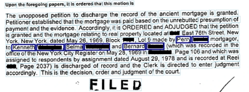
You can see the results in Figure 1. We can later use this layout information for many purposes.
Based on the content, we can decide whether any block in a given layout contains the title. For document classification based on title, it seems that predicting document class based only on the detected title would be as good as based on the document content. The only problem occurs when there are no document titles, which unfortunately happens often.
Overall, mixing layout information with the text content is definitely a way to go, because layout seems to be an integral part of a document, fulfilling not only the cosmetic needs but also storing substantive information. Imagine you are reading these documents as plain text in notepad - some signs, dates, addresses, are impossible to distinguish without localizations and correctly interpreted order of text lines.
The entire pipeline of classification is visualized in Figure 2.
Validation
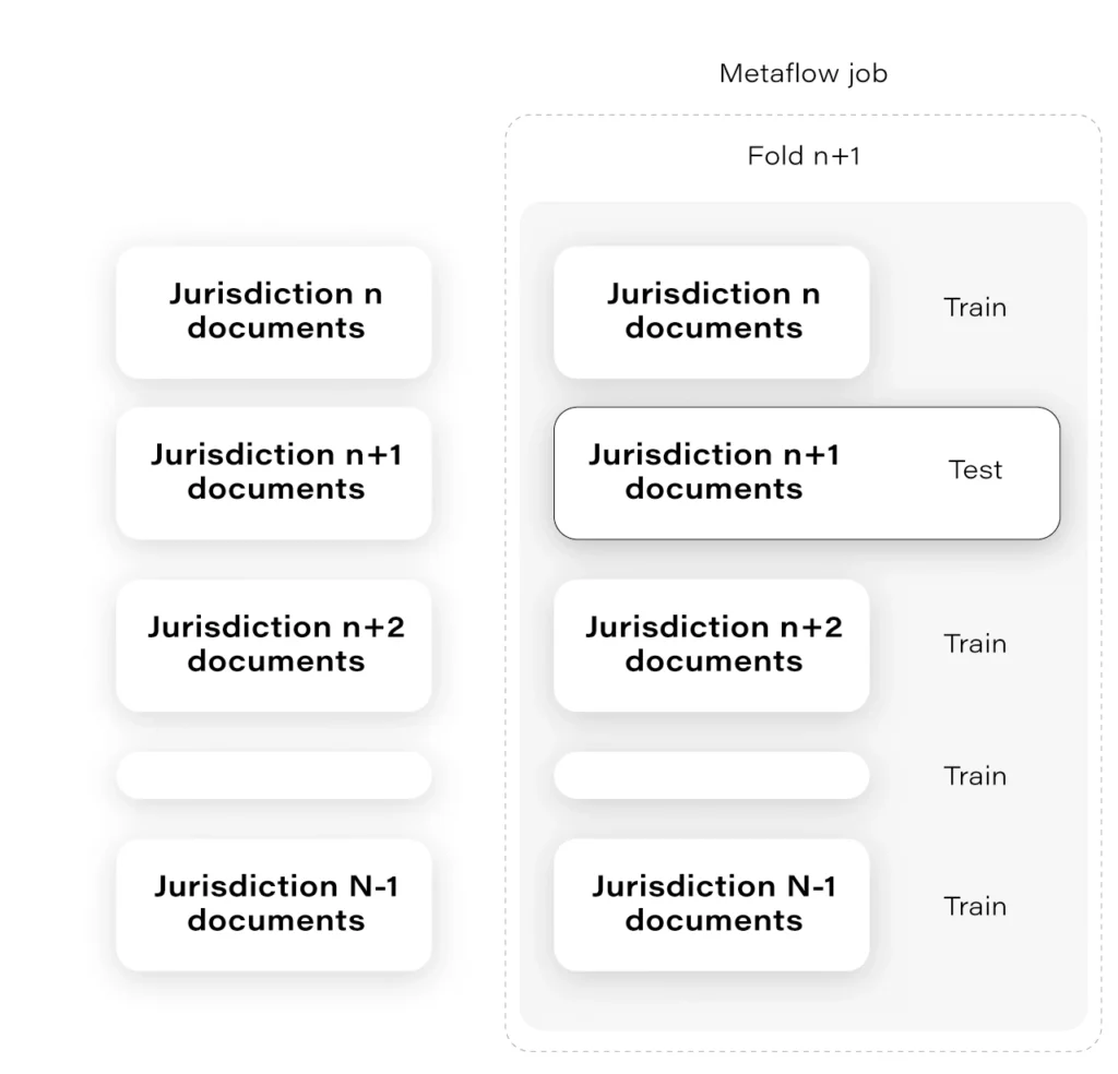
We incorporated the Metaflow python package for this project. It is a complicated technology that does not always work fluently but overall we think it gave us useful horizontal scalability (some time-consuming processes) and facilitated the cooperation between team members.
The interesting example of Metaflow usage is as follows: at some time, we had to assure that the number of jurisdictions that we had in our trainset is enough for the model to generalize over all jurisdictions.
Are we sure the mortgage from some small jurisdiction in Alaska will work even though most of our documents come from, let’s say, West Side?
The solution to that was to prepare the “leave-one-out" cross-validation in a way that we hold documents from one jurisdiction as a validation set. Having a lot of jurisdictions, we had to choose N of them. Each fold was tested on a remote machine independently and in parallel, which was largely facilitated thanks to Metaflow. Check the Figure 3.
Next
Classification is a crucial component of our system and allows us to take further steps. Having solid fundamentals, after the classifier routing, we can run the next services – the finders .
Train your computer with the Julia programming language - introduction
As the Julia programming language is becoming very popular in building machine learning applications, we explain its advantages and suggest how to leverage them.
Python and its ecosystem have dominated the machine learning world – that’s an undeniable fact. And it happened for a reason. Ease of use and simple syntax undoubtedly contributed to still growing popularity. The code is understandable by humans, and developers can focus on solving an ML problem instead of focusing on the technical nuances of the language. But certainly, the most significant source of technology success comes from community effort and the availability of useful libraries.
In that context, the Python environment really shines. We can google in five seconds a possible solution for a great majority of issues related to the language, libraries, and useful examples, including theoretical and practical aspects of our intelligent application or scientific work. Most of the machine learning related tutorials and online courses are embedded in the Python ecosystem. If some ML or AI algorithm is worth of community’s attention, there is a huge probability that somebody implemented it as a Python open-source library.
Python is also the "Programming Language of the 2020" award winner. The award is given to the programming language that has the highest rise in ratings in a year based on the TIOBE programming community index (a measure of the popularity of programming languages). It is worth noting that the rise of Python language popularity is strongly correlated with the rise of machine learning popularity.
Equipped with such great technology, why still are we eager to waste a lot of our time looking for something better? Except for such reasons as being bored or the fact that many people don’t like snakes (although the name comes from „Monty Python’s Flying Circus”, a python still remains a snake). We think that the answer is quite simple: because we can do it better.
From Python to Julia
To understand that there is a potential to improve, we can go back to the early nineties when Python was created. It was before 3rd wave of artificial intelligence popularity and before the exponential increase in interest in deep learning. Some hard-to-change design decisions that don’t fit modern machine learning approaches were unavoidable. Python is old, it’s a fact, a great advantage, but also a disadvantage. A lot of great and groundbreaking things happened from the times when Python was born.
While Python has dominated the ML world, a great alternative has emerged for anyone who expects more. The Julia Language was created in 2009 by a four-person team from MIT and released in 2012. The authors wanted to address the shortcomings in Python and other languages. Also, as they were scientists, they focused on scientific and numerical computation, hitting a niche occupied by MATLAB, which is very good for that application but is not free and not open source. The Julia programming language combines the speed of C with the ease of use of Python to satisfy both scientists and software developers. And it integrates with all of them seamlessly.
In the following sections, we will show you how the Julia Language can be adapted to every Machine Learning problem . We will cover the core features of the language shown in the context of their usefulness in machine learning and comparison with other languages. A short overview of machine learning tools and frameworks available in Julia is also included. Tools for data preparation, visualization of results, and creating production pipelines also are covered. You will see how easily you can use ML libraries written in other languages like Python, MATLAB, or C/C++ using powerful metaprogramming features of the Julia language. The last part presents how to use Julia in practice, both for rapid prototyping and building cloud-based production pipelines.
The Julia language
Someone said if Python is a premium BMW sedan (petrol only, I guess, eventual hybrid) then Julia is a flagship Tesla. BMW has everything you need, but more and more people are buying Tesla. I can somehow agree with that, and let me explain the core features of the language which makes Julia so special and let her compete for a place in the TIOBE ranking with such great players as LISP, Scala, or Kotlin (31st place in March 2021).
Unusual JIT/AOT complier
Julia uses the LLVM compiler framework behind the scenes to translate very simple and dynamic syntax into machine code. This happens in two main steps. The first step is precompilation, before final code execution, and what may be surprising this it actually runs the code and stores some precompilation effects in the cache. It makes runtime faster but slower building – usually this is an acceptable cost.
The second step occurs in runtime. The compiler generates code just before execution based on runtime types and static code analysis. This is not how traditional just-in-time compilers work e.g., in Java. In “pure” JIT the compiler is not invoked until after a significant number of executions of the code to be compiled. In that context, we can say that Julia works in much the same way as C or C++. That’s why some people call Julia compiler a just-ahead-of-time compiler, and that’s why Julia can run near as fast as C in many cases while remaining a dynamic language like Python. And this is just awesome.
Read-eval-print loop
Read-eval-print loop (REPL) is an interactive command line that can be found in many modern programming languages. But in the case of Julia, the REPL can be used as the real heart of the entire development process. It lets you manage virtual environments, offers a special syntax for the package manager, documentation, and system shell interactions, allows you to test any part of your code, the language, libraries, and many more.
Friendly syntax
The syntax is similar to MATLAB and Python but also takes the best of other languages like LISP. Scientists will appreciate that Unicode characters can be used directly in source code, for example, this equation: f(X,u,σᵀ∇u,p,t) = -λ * sum(σᵀ∇u.^2)
is a perfectly valid Julia code. You may notice how cool it can be in terms of machine learning. We use these symbols in machine learning related books and articles, why not use them in source code?
Optional typing
We can think of Julia as dynamically typed but using type annotation syntax, we can treat variables as being statically typed, and improve performance in cases where the compiler could not automatically infer the type. This approach is called optional typing and can be found in many programming languages. In Julia however, if used properly, can result in a great boost of performance as this approach fits very well with the way Julia compiler works.
A ‘Glue’ language
Julia can interface directly with external libraries written in C, C++, and Fortran without glue code. Interface with Python code using PyCall library works so well that you can seamlessly use almost all the benefits of great machine learning Python ecosystem in Julia project as if it were native code! For example, you can write:
np = pyimport(numpy)
and use numpy in the same way you do with Python using Julia syntax. And you can configure a separate miniconda Python interpreter for each project and set up everything with one command as with Docker or similar tools. There are bindings to other languages as well e.g., Java, MATLAB, or R.
Julia supports metaprogramming
One of Julia's biggest advantages is Lisp-inspired metaprogramming. A very powerful characteristic called homoiconicity explained by a famous sentence: “code is data and data is code” allows Julia programs to generate other Julia programs, and even modify their own code. This approach to metaprogramming gives us so much flexibility, and that’s how developers do magic in Julia.
Functional style
Julia is not an object-oriented language. Something like a model.fit() function call is possible (Julia is very flexible) but not common in Julia. Instead, we write fit(model) , and it's not about the syntax, but it is about the organization of all code in our program (modules, multiple dispatches, functions as a first-class citizen, and many more).
Parallelization and distributed computing
Designed with ML in mind, Julia focusses on the scientific computing domain and its needs like parallel, distributed intensive computation tasks. And the syntax is very easy for local or remote parallelism.
Disadvantages
Well, it might be good if the compiler wasn't that slow, but it keeps getting better. Sometimes REPL could be faster, but again it’s getting better, and it depends on the host operating system.
Conclusion
By concluding this section, we would like to demonstrate a benchmark comparing several popular languages and Julia. All language benchmarks should be treated not too seriously, but they still give an approximate view of the situation.
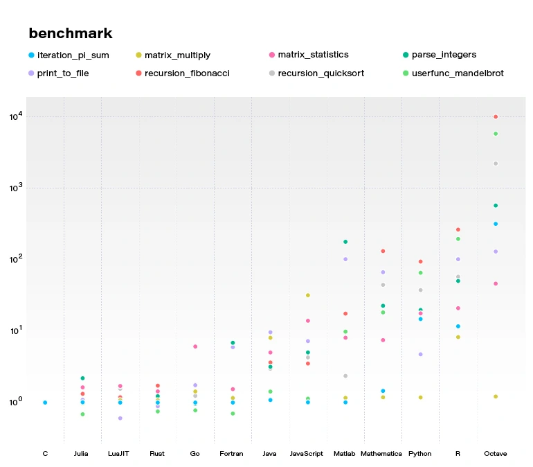
Julia becomes more and more popular. Since the 2012 launch, Julia has been downloaded over 25,000,000 times as of February 2021, up by 87% in a year.
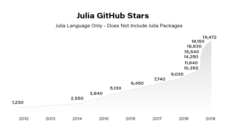
In the next article, we focus on using Julia in building Machine Learning models. You can also check our guide to getting started with the language .
Introduction to building intelligent document processing systems
Building Intelligent Document Processing systems for financial institutions is challenging. In this article, we share our approach to developing an IDP solution that goes far beyond a simple NLP task.
The series about Intelligent Document Processing (IDP) consists of 3 parts:
- Problem definition and data
- Classification and validation
- Entities finders
Building intelligent document processing systems - problem introduction
The selected domain that could be improved with AI was mortgage filings . These filings are required for mortgages to be serviced or transferred and are jurisdiction-specific. When a loan is serviced, many forms are filed with jurisdictions, banks, servicing companies, etc. These forms must be filed promptly, correctly, and accurately. Many of these forms are actual paper as only a relatively small number of jurisdictions allow for e-sign.
The number of types of documents is immense. For example, we are looking at MSR Transfers, lien release, lien perfection, servicing transfer, lien enforcement, lien placement, foreclosure, forbearance, short sell, etc. All of these procedures have more than one form and require specific timeframes for not only filing but also follow-up. Most jurisdictions are extremely specific on the documents and their layout. Ranging from margins to where the seals are placed to a font to sizing to wording. It can change between geographically close jurisdictions.
What may be surprising, these documents, usually paper, are sent to the centers to be sorted and scanned. The documents are visually inspected by a human. They decide not only further processing of the documents but sometimes need to extract or tag some knowledge at the stage of routing. This process seems incredibly laborious considering the fact that a large organization can process up to tens of thousands of documents per day!
AI technology, as its understanding and trust grows, naturally finds a place in similar applications, automating subsequent tasks, one by one. There are many places waiting for technological advancement, and here are some ideas on how it can be done.
Overview
There are a few crucial components in the prepared solution
- OCR
- Documents classification
- Jurisdiction recognition
- Property addresses
- Party names and roles
- Document and file date
Each of them has some specific aspects that have to be handled, but all of them (except OCR) fall into one of 2 classical Natural Language Processing tasks: classification and Named Entity Recognition (NER).
OCR
There are a lot of OCRs that can transcribe the text from a document. Contrary to what we know after working on VIN Recognition System , the available OCRs are probably designed and are doing well on random documents of various kinds.
On the other hand, having some possibilities – Microsoft Computer Vision, AWS Textract, Google Cloud Vision, open-source Tesseract, naming a few, how to choose the best one? Determining the solution that fits best in our needs is a tough decision on its own. It requires well-structured experiments.
- We needed to prepare test sets to benchmark overall accuracy
- We needed to analyze the performance on handwriting
The results showed huge differences between the services, both in terms of accuracy on regular and hand-written text.
The best services we found were Microsoft Computer Vision, AWS Textract, and Google Cloud Vision. On 3 sets, they achieved the following results:
AWS Textract Microsoft CV Google CV Set 1 66.4 95.8 93.1 Set 2 87.2 96.5 91.8 Set 3 78.0 92.6 93.8 % of OCR results on different benchmarks
Hand-written text works on its own terms. As often in the real world, any tool has weaknesses, and the performance on printed text is somehow opposite to the performance on the hand-written text. In summary, OCRs have different characteristics in terms of output information, recognition time, detection, and recognition accuracy. There are at best 8% errors, but some services work as badly as recognizing 25% of words wrongly.
After selecting OCR, we had to generate data for classifiers. Recognizing tons of documents is a time-consuming process (the project team spent an extra month on the character recognition itself.) After that step, we could collect the first statistics and describe the data.
Data diversity
We collected over 80000 documents. The average file had 4.3 pages. Some of them longer than 10 pages, with a record holder of 96 pages.
Take a look at the following documents – Document A and Document B. They are both of the same type – Bill of Sale!

- Half of document A is hand-written, while the other has only signatures
- There is just a brief detail about the selling process on Doc A, whereas on the other there are a lot of details about the truck inspection
- The sold vehicle in document B is described in the table
- Only the day in the document date of document B is hand-written
- There is a barcode on the Doc A
- The B document has 300% more words than the A
Also, we find a visual impression of these documents much different.
How can the documents be so different? The types of documents are extremely numerous and varied, but also are constantly being changed and added by the various jurisdictions. Sometimes they are sent together with the attachments, so we have to distinguish the attachment from the original document.
There are more than 3000 jurisdictions in the USA. Only a few administrative jurisdictions share mortgage fillings. Fortunately, we could focus on present-day documents, but it happens that some of the documents have to be processed that are more than 30 years old.
Some documents were well structured: each interesting value was annotated with a key, everything in tables. It happened, however, that a document was entirely hand-written. You can see some documents in the figures. Take a note that some information on the first is just a work marked with a circle!


Next steps
The obtained documents were just the fundamentals for the next research. Such a rich collection enabled us to take the next steps , even though the variety of documents was slightly frightening. Did we manage to use the gathered documents for a working system?
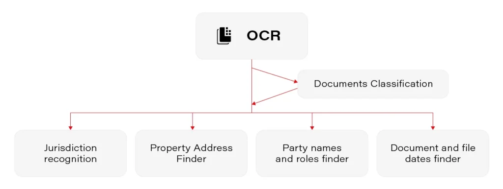
Key insights from Insurance Innovators USA 2021
Insurance Innovators USA 2021, organized by Market Force Live, provided us with engaging sessions and insights into trends shaping the industry. We sum up key points and share our thoughts regarding commonly discussed predictions.
External sources of innovation
In a traditional approach, innovation was supposed to be driven by the internal capacity of an organization. So, achieved goals in innovation and R&D used to be an internal cost/benefit relation. That paradigm has started to shift in recent years and was clearly accelerated by the unexpected pressure from COVID pandemic.
Insurance companies understand the importance of collaborating with external experts to drive innovation. Both InsurTechs and technology vendors they choose to collaborate with, provide them with a fresh take on your organization and processes, and that leads to unlocking innovation. Staying open-minded, monitoring what the market has to offer, and evaluating new products and services enable organizations to be agile and competitive.
Amazon is the new customer experience baseline
The insurance industry drags behind many other industry sectors in the digital transformation. But the rise of customer-centric technology providers encourages the industry to reconsider its stance. Until recently, customers tended to remain with their providers for long periods because it was easier to do a renewal than to shop for a policy and face all the hassle.
Now that the InsurTechs are here, insurance companies face the same dilemma the retail industry has a couple of years back. They either adopt the customer-centric, digital approach to servicing their customers, or they will lose market share. The days when customers went to see their insurance agents are mostly gone now. In the age of Amazon, insurance companies must offer a buying experience and a personalized relationship that will make finding, buying and renewing insurance simple and pleasant.
Covid-19 accelerated virtual inspections
Prior to Covid-19, only the largest companies advanced in their digital transformation journey leveraged virtual inspections. As no one expected that a global pandemic would hit and force everyone to retreat to virtual channels, they mainly used virtual inspections to enhance productivity and to speed up claims processing. Companies like Allstate that have implemented virtual inspections back in 2016 ( you can read here how Grape Up helped Allstate build their solution ) have simply scaled up the teams and made it their no.1 channel of communication.
For companies that have not considered VI before, it took some time to launch the virtual inspection capability, but fortunately, with SaaS solutions available, the adoption was relatively easy. What seems to be certain at this point, according to the conference panelists, is that the virtual inspections are here to stay. Even with the pandemic gone and social interactions resumed, it is unlikely the insurance companies will want to go back to in-person inspections, and more importantly, that the customers will.
Embedded insurance is growing
Embedded insurance is one of the hot topics of 2021 that may well change forever the adage saying insurance is something a person needs rather than wants. With the development of connectivity, IT architectures, APIs, and digital ecosystems, embedded insurance has the potential to provide a one-stop-shop experience for customers buying new products. The embedded insurance model installs the coverage within the purchase of a product. That means the insurance is not sold to the customer at some point in the future but is instead provided as a native feature of the product.
That way a new smartphone is covered for theft and damage right from the get-go. For insurance companies, this new way of doing business promises a variety of new opportunities to develop, enter, and target insurance segments they have not operated in before.
From the technology standpoint, it seems clear that all these trends will drive insurance companies to further develop their cloud and data capabilities . The ability to perform operations on data in near real-time will be the key to sustaining and growing the customer-centric approach that is necessary if carriers want to remain competitive.
Getting started with the Julia language
Are you looking for a programming language that is fast, easy to start with, and trending? The Julia language meets the requirements. In this article, we show you how to take your first steps.
What is the Julia language?
Julia is an open-source programming language for general purposes. However, it is mainly used for data science, machine learning , or numerical and statistical computing. It is gaining more and more popularity. According to the TIOBE index, the Julia language jumped from position 47 to position 23 in 2020 and is highly expected to head towards the top 20 next year.
Despite the fact Julia is a flexible dynamic language, it is extremely fast. Well-written code is usually as fast as C, even though it is not a low-level language. It means it is much faster than languages like Python or R, which are used for similar purposes. High performance is achieved by using type interference and JIT (just-in-time) compilation with some AOT (ahead-of-time) optimizations. You can directly call functions from other languages such as C, C++, MATLAB, Python, R, FORTRAN… On the other hand, it provides poor support for static compilation, since it is compiled at runtime.
Julia makes it easy to express many object-oriented and functional programming patterns. It uses multiple dispatches, which is helpful, especially when writing a mathematical code. It feels like a scripting language and has good support for interactive use. All those attributes make Julia very easy to get started with and experiment with.
First steps with the Julina language
- Download and install Julia from Download Julia .
- (Optional - not required to follow the article) Choose your IDE for the Julia language. VS Code is probably the most advanced option available at the moment of writing this paragraph. We encourage you to do your research and choose one according to your preferences. To install VSCode, please follow Installing VS Code and VS Code Julia extension .
Playground
Let’s start with some experimenting in an interactive session. Just run the Julia command in a terminal. You might need to add Julia's binary path to your PATH variable first. This is the fastest way to learn and play around with Julia.
C:\Users\prso\Desktop>julia
_
_ _ _(_)_ | Documentation: https://docs.julialang.org
(_) | (_) (_) |
_ _ _| |_ __ _ | Type "?" for help, "]?" for Pkg help.
| | | | | | |/ _` | |
| | |_| | | | (_| | | Version 1.5.3 (2020-11-09)
_/ |\__'_|_|_|\__'_| | Official https://julialang.org/ release
|__/ |
julia> println("hello world")
hello world
julia> 2^10
1024
julia> ans*2
2048
julia> exit()
C:\Users\prso\Desktop>
To get a recently returned value, we can use the ans variable. To close REPL, use exit() function or Ctrl+D shortcut.
Running the scripts
You can create and run your scripts within an IDE. But, of course, there are more ways to do so. Let’s create our first script in any text editor and name it: example.jl.
x = 2
println(10x)
You can run it from REPL:
julia> include("example.jl")
20
Or, directly from your system terminal:
C:\Users\prso\Desktop>julia example.jl
20
Please be aware that REPL preserves the current state and includes statement works like a copy-paste. It means that running included is the equivalent of typing this code directly in REPL. It may affect your subsequent commands.
Basic types
Julia provides a broad range of primitive types along with standard mathematical functions and operators. Here’s the list of all primitive numeric types:
- Int8, UInt8
- Int16, UInt16
- Int32, UInt32
- Int64, UInt64
- Int128, UInt128
- Float16
- Float32
- Float64
A digit suffix implies several bits and a U prefix that is unsigned. It means that UInt64 is unsigned and has 64 bits. Besides, it provides full support for complex and rational numbers.
It comes with Bool , Char , and String types along with non-standard string literals such as Regex as well. There is support for non-ASCII characters. Both variable names and values can contain such characters. It can make mathematical expressions very intuitive.
julia> x = 'a'
'a': ASCII/Unicode U+0061 (category Ll: Letter, lowercase)
julia> typeof(ans)
Char
julia> x = 'β'
'β': Unicode U+03B2 (category Ll: Letter, lowercase)
julia> typeof(ans)
Char
julia> x = "tgα * ctgα = 1"
"tgα * ctgα = 1"
julia> typeof(ans)
String
julia> x = r"^[a-zA-z]{8}$"
r"^[a-zA-z]{8}$"
julia> typeof(ans)
Regex
Storage: Arrays, Tuples, and Dictionaries
The most commonly used storage types in the Julia language are: arrays, tuples, dictionaries, or sets. Let’s take a look at each of them.
Arrays
An array is an ordered collection of related elements. A one-dimensional array is used as a vector or list. A two-dimensional array acts as a matrix or table. More dimensional arrays express multi-dimensional matrices.
Let’s create a simple non-empty array:
julia> a = [1, 2, 3]
3-element Array{Int64,1}:
1
2
3
julia> a = ["1", 2, 3.0]
3-element Array{Any,1}:
"1"
2
3.0
Above, we can see that arrays in Julia might store Any objects. However, this is considered an anti-pattern. We should store specific types in arrays for reasons of performance.
Another way to make an array is to use a Range object or comprehensions (a simple way of generating and collecting items by evaluating an expression).
julia> typeof(1:10)
UnitRange{Int64}
julia> collect(1:3)
3-element Array{Int64,1}:
1
2
3
julia> [x for x in 1:10 if x % 2 == 0]
5-element Array{Int64,1}:
2
4
6
8
10
We’ll stop here. However, there are many more ways of creating both one and multi-dimensional arrays in Julia.
There are a lot of built-in functions that operate on arrays. Julia uses a functional style unlike dot-notation in Python. Let’s see how to add or remove elements.
julia> a = [1,2]
2-element Array{Int64,1}:
1
2
julia> push!(a, 3)
3-element Array{Int64,1}:
1
2
3
julia> pushfirst!(a, 0)
4-element Array{Int64,1}:
0
1
2
3
julia> pop!(a)
3
julia> a
3-element Array{Int64,1}:
0
1
2
Tuples
Tuples work the same way as arrays. A tuple is an ordered sequence of elements. However, there is one important difference. Tuples are immutable. Trying to call methods like push!() will result in an error.
julia> t = (1,2,3)
(1, 2, 3)
julia> t[1]
1
Dictionaries
The next commonly used collections in Julia are dictionaries. A dictionary is called Dict for short. It is, as you probably expect, a key-value pair collection.
Here is how to create a simple dictionary:
julia> d = Dict(1 => "a", 2 => "b")
Dict{Int64,String} with 2 entries:
2 => "b"
1 => "a"
julia> d = Dict(x => 2^x for x = 0:5)
Dict{Int64,Int64} with 6 entries:
0 => 1
4 => 16
2 => 4
3 => 8
5 => 32
1 => 2
julia> sort(d)
OrderedCollections.OrderedDict{Int64,Int64} with 6 entries:
0 => 1
1 => 2
2 => 4
3 => 8
4 => 16
5 => 32
We can see, that dictionaries are not sorted. They don’t preserve any particular order. If you need that feature, you can use SortedDict .
julia> import DataStructures
julia> d = DataStructures.SortedDict(x => 2^x for x = 0:5)
DataStructures.SortedDict{Any,Any,Base.Order.ForwardOrdering} with 6 entries:
0 => 1
1 => 2
2 => 4
3 => 8
4 => 16
5 => 32
DataStructures is not an out-of-the-box package. To use it for the first time, we need to download it. We can do it with a Pkg package manager.
julia> import Pkg; Pkg.add("DataStructures")
Sets
Sets are another type of collection in Julia. Just like in many other languages, Set doesn’t preserve the order of elements and doesn’t store duplicated items. The following example creates a Set with a specified type and checks if it contains a given element.
julia> s = Set{String}(["one", "two", "three"])
Set{String} with 3 elements:
"two"
"one"
"three"
julia> in("two", s)
true
This time we specified a type of collection explicitly. You can do the same for all the other collections as well.
Functions
Let’s recall what we learned about quadratic equations at school. Below is an example script that calculates the roots of a given equation: ax2+bx+c .
discriminant(a, b, c) = b^2 - 4a*c
function rootsOfQuadraticEquation(a, b, c)
Δ = discriminant(a, b, c)
if Δ > 0
x1 = (-b - √Δ)/2a
x2 = (-b + √Δ)/2a
return x1, x2
elseif Δ == 0
return -b/2a
else
x1 = (-b - √complex(Δ))/2a
x2 = (-b + √complex(Δ))/2a
return x1, x2
end
end
println("Two roots: ", rootsOfQuadraticEquation(1, -2, -8))
println("One root: ", rootsOfQuadraticEquation(2, -4, 2))
println("No real roots: ", rootsOfQuadraticEquation(1, -4, 5))
There are two functions. The first one is just a one-liner and calculates a discriminant of the equation. The second one computes the roots of the function. It returns either one value or multiple values using tuples.
We don’t need to specify argument types. The compiler checks those types dynamically. Please take note that the same happens when we call sqrt() function using a √ symbol. In that case, when the discriminant is negative, we need to wrap it with a complex()function to be sure that the sqrt() function was called with a complex argument.
Here is the console output of the above script:
C:\Users\prso\Documents\Julia>julia quadraticEquations.jl
Two roots: (-2.0, 4.0)
One root: 1.0
No real roots: (2.0 - 1.0im, 2.0 + 1.0im)
Plotting
Plotting with the Julia language is straightforward. There are several packages for plotting. We use one of them, Plots.jl.
To use it for the first, we need to install it:
julia> using Pkg; Pkg.add("Plots")
After the package was downloaded, let’s jump straight to the example:
julia> f(x) = sin(x)cos(x)
f (generic function with 1 method)
julia> plot(f, -2pi, 2pi)
We’re expecting a graph of a function in a range from -2π to 2π. Here is the output:
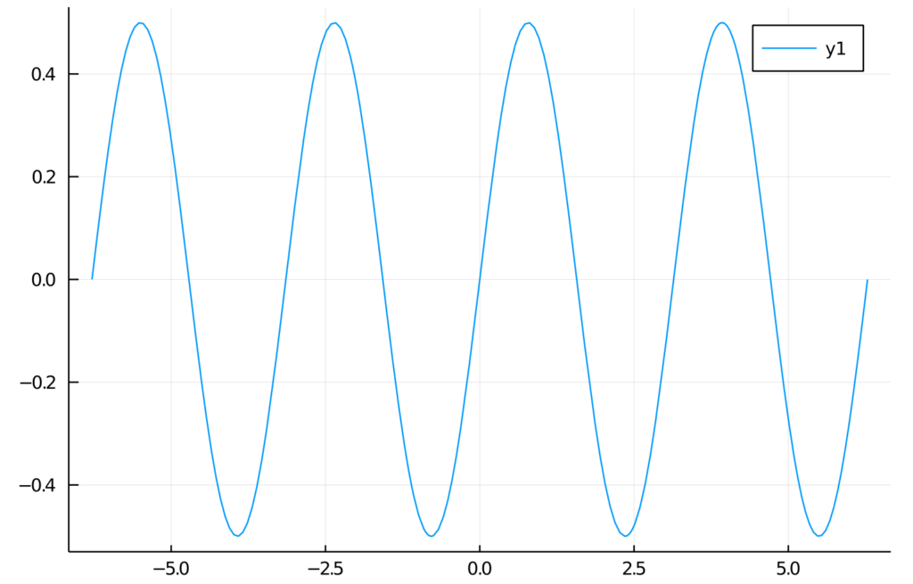
Summary and further reading
In this article, we learned how to get started with Julia. We installed all the required components. Then we wrote our first “hello world” and got acquainted with basic Julia elements.
Of course, there is no way to learn a new language from reading one article. Therefore, we encourage you to play around with the Julia language on your own.
To dive deeper, we recommend reading the following sources:
Automating your enterprise infrastructure. Part 2: Cloud Infrastructure as code in practice (AWS Cloud Formation example)
Given that you went through Part 1 of the Infrastructure automation guide, and you already know basic Infrastructure as Code and AWS Cloud Formation concepts, we can proceed with getting some hands-on experience!
Learn more about services provided by Grape Up
You are at Grape Up blog, where our experts share their expertise gathered in projects delivered for top enterprises. See how we work.
Enabling the automotive industry to build software-defined vehicles
Empowering insurers to create insurance telematics platforms
Providing AI & advanced analytics consulting
Note that in this article, we’ll build Infrastructure as Code scripts for the infrastructure described by Michal Kapiczynski in the series of mini-articles .
HINT Before we begin:
If you’re building your Cloud Formation scripts from scratch, we highly recommend starting with spinning the infrastructure manually from the AWS console, and later on, use the AWS CLI tool to get a ‘description’ of the resource. The output will show you the parameters and their values that were used to create the resource.
E.g use:
aws ec2 describe-instances
to obtain properties for EC2 instances.
Let's recall what is our target state:
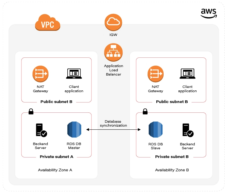
As already mentioned in the first part of the automation guide , we've split the infrastructure setup into two Templates (scripts). Let’s start with the first one, called infra-stack, as it contains Architecture scaffolding resources:
- VPC
- Subnets
- Internet gateway
- Elastic IP
- NAT
- Route Tables
Note: All of the Cloud Formation scripts presented below and even more are publicly accessible in this GitHub repository .
VPC
The backbone - Virtual private cloud, in fact a network that hosts all of our resources. Cloud Formation definition for this one is a simple one. See:
UserManagementVpc:
Type: AWS::EC2::VPC
Properties:
CidrBlock: "10.0.0.0/22"
Tags:
- Key: "Name"
Value: "UserManagementVpc"
Just a few lines of code. The first line defines the Amazon resource name, we’ll use this name later on to reference the VPC. Type specifies whether this is VPC, Subnet, EC2 VM, etc. The Properties section contains a set of configuration key-value pairs fixed for a particular resource. The only required property that we define here is CidrBlock of our VPC. Note the network mask (256.256. 252.0 ). Additionally, we can specify a Name Tag that might help us to quickly find our VPC amid the VPC list in the AWS console.
Subnets
As stated above, we’ll need 4 subnets. Specifically, one public and one private network subnet in Availability Zone A. The same goes for AZ B. Let’s see public subnet A definition:
PubSubnetA:
Type: AWS::EC2::Subnet
Properties:
AvailabilityZone: !Sub '${Region}a'
CidrBlock: 10.0.0.0/24
Tags:
- Key: 'Name'
Value: 'PubSubnetA'
VpcId: !Ref UserManagementVpc
When specifying AvailabilityZone, we can use !Sub function to substitute Region script parameter variable name with the actual value and at the same time, concatenate it with ‘a’ suffix. This is to have an actual AWS Region name. So, e.g. taking the Region default value, the actual value for AvailabilityZone in the figure above is “eu-central-1a“.
Next, we have to specify CidrBock of the subnet. This one is easy, though note that subnet cidr should be ‘within’ VPC cidr block.
Last but not least, VpcId . At the time we write the script, we don’t know the actual VPC identifier, that’s why we have to reference ( !Ref ) VPC by its name ( UserManagementVpc) .
Both of the functions - !Sub and !Ref are so-called intrinsic function references built-in into cloud formation service. More on that here .
We won’t go through the rest of the Subnet definitions, these are basically the same, the only thing that changes is AvailabilityZone suffix and CirdBlock. You can find these definitions in the Github repository .
Internet gateway
This one seems to be a simple one:
IGW:
Type: AWS::EC2::InternetGateway
Properties:
Tags:
- Key: "Name"
Value: "MyIGW"
The only required field is Type. Not so fast though. As we already know IGW should be attached to a specific VPC, but there is no VPC reference here! Here comes the other Resource called VpcGatewayAttachment:
IgwAttachment:
Type: AWS::EC2::VPCGatewayAttachment
Properties:
InternetGatewayId: !Ref IGW
VpcId: !Ref UserManagementVpc
As we clearly see, this one is responsible for the association between IGW and VPC. Same as in Subnet definition, we can reference these by name using !Ref.
Elastic IP
Now, let’s take care of the prerequisites for NAT setup. We ought to set up Elastic IP that NAT can reference later on. We need two of these for each AZ:
EIPa:
Type: AWS::EC2::EIP
Properties:
Tags:
- Key: "Name"
Value: "EIPa"
Note ‘a’ suffix which indicates target AZ for the EIP.
NAT (Network Address Translation) gateway
Since we have prerequisites provisioned, we can now set up two NAT Gateway instances in our public subnets:
NATa:
Type: AWS::EC2::NatGateway
Properties:
AllocationId: !GetAtt EIPa.AllocationId
SubnetId: !Ref PubSubnetA
Tags:
- Key: "Name"
Value: "NATa"
As you - the careful reader - noted, to obtain the value for AllocationId we used yet another intrinsic function reference, Fn::GetAtt. This use facilitates obtaining Elastic IP attribute - AllocationId . Next, we reference the target SubnetId . As always, we have to remember to spin up twin NAT in b AZ.
Route tables
Things get a little bit messy here. First, we’ll create our Main Route table that will hold the rules for our public subnets.
MainRT:
Type: AWS::EC2::RouteTable
Properties:
Tags:
- Key: "Name"
Value: "MainRT"
VpcId: !Ref UserManagementVpc
This is where our CloudFormation IoC script turns out to be more complicated than a simple setup through Amazon console.
Turns out that Rules specification is yet another resource:
MainRTRoute:
Type: AWS::EC2::Route
Properties:
DestinationCidrBlock: 0.0.0.0/0
GatewayId: !Ref IGW
RouteTableId: !Ref MainRT
The essence of this is the DestinationCidrBlock configuration. As you see, we’ve set it to 0.0.0.0/0, which means that we allow for unrestricted access to all IPv4 addresses. Also, we need to reference our Internet gateway and instruct our Route resource to attach itself to the MainRT .
Unfortunately, Route Table configuration doesn’t end here. Additionally, we have to associate RouteTable with the subnet. As we aforementioned, we’ll associate MainRT with our public subnets. See:
MainRTSubnetAAssociation:
Type: AWS::EC2::SubnetRouteTableAssociation
Properties:
RouteTableId: !Ref MainRT
SubnetId: !Ref PubSubnetA
Remember to do the same for public subnet b!
For private subnets, the story goes all over again. We need yet another Route table, SubnetRouteTableAssociation, and Route definitions. But in this case, we will enforce all outgoing traffic to be routed through NAT Gateways.
NOTE: In production environments, it’s considered good practice to disable internet access in private networks!
Outputs section
Besides actual resources, the script also defines the Outputs section. The section defines what Stack information may be exposed for others Stacks. This mechanism will allow us to - later on - reference VPC and Subnet identifiers in the second stack.
EC2, Database & Load Balancer stack
Next in line, vm-and-db-stack, it contains declarative definitions of:
- AWS KeyPair - prerequisite
- EC2
- Multi-AZ Database setup
- Load Balancer - AWS Application Elastic Load balancer
The script accepts three parameters (no worry - default values are included):
- NetworkStackName - the name of the infrastructure stack that we created in the previous step.
- DBPass - self-explanatory.
AvailabilityZone - target AWS Availability Zone for the stack. Note that the value has to be coherent with the AZ parameter value specified when running the infrastructure stack script.
AWS KeyPair - prerequisite
Before we proceed with this stack, there is one resource that you, as an account owner, have to provision manually. The thing is AWS KeyPair. Long story short, it’s AWS equivalent to private & public asymmetric cryptographic keys. We’ll need these to access Virtual Machines running in the cloud!
You can do it either through AWS console or use aws cli tool:
  $ aws ec2 create-key-pair --key-name=YourKeyPairName \
  --query ‘KeyMaterial’ --output text > MySecretKey.pem
Remember the key name since we’ll reference it later.
EC2
Eventually, we need some VM to run our application! Let’s see an example configuration for our EC2 running in a private subnet in AZ a:
ServerAEC2:
Type: AWS::EC2::Instance
Properties:
AvailabilityZone: !Sub '${Region}a'
KeyName: training-key-pair
BlockDeviceMappings:
- DeviceName: '/dev/sda1'
Ebs:
VolumeSize: 8 # in GB
ImageId: 'ami-03c3a7e4263fd998c' # Amazon Linux 2 AMI (64-bit x86)
InstanceType: 't3.micro' # 2 vCPUs & 1 GiB
NetworkInterfaces:
- AssociatePublicIpAddress: false
PrivateIpAddress: '10.0.1.4'
SubnetId:
Fn::ImportValue:
Fn::Sub: "${InfrastructureStackName}-PrivSubnetA"
DeviceIndex: '0'
Description: 'Primary network interface'
GroupSet:
- !Ref ServerSecurityGroup
Tags:
- Key: Name
Value: ServerAEC2
This one is a little bit longer. First, as aforementioned, we reference our KeyPair name ( KeyName parameter) that we’ve created as a prerequisite.
There comes persistence storage configuration - BlockDeviceMappings . We state that we’re going to need 8 GB of storage, attached to /dev/sda1 partition.
Next, we choose the operating system - ImageId . I’ve used Amazon Linux OS, but you can use whatever AMI you need.
In the networking section ( NetworkInterfaces), we’ll link our EC2 instance with the subnet. SubnetId sub-section uses another intrinsic function - Fn::ImportValue . We use it to capture the output exported by the infrastructure stack ( Outputs section). By combining it with Fn::Sub we can easily reference private subnet ‘a’.
NetworkInterfaces property also contains a list named GroupSet , although the name might not indicate so, this is a list containing Security Group references that should be attached to our EC2. We’ll follow up with the Security Group resource in the next section.
Remember to follow this pattern to create a Client facing EC2 VMs in public subnets. These are pretty much the same, the only notable difference is security groups. For client-facing machines, we’ll reference ClientSecurityGroup .
Security Groups
Security is undoubtedly one of the most significant topics for modern Enterprises. Having it configured the right way will prevent us from pervasive data breaches .
ServerSecurityGroup:
Type: AWS::EC2::SecurityGroup
Properties:
GroupDescription: 'Server security group'
GroupName: 'ServerSecurityGroup'
SecurityGroupIngress:
- CidrIp: '0.0.0.0/0'
IpProtocol: TCP
FromPort: 22
ToPort: 22
- SourceSecurityGroupId: !Ref LoadBalancerSecurityGroup
IpProtocol: TCP
FromPort: 8080
ToPort: 8080
SecurityGroupEgress:
- CidrIp: '0.0.0.0/0' # Not for Prod
IpProtocol: -1 # Allow all
VpcId:
Fn::ImportValue:
Fn::Sub: "${InfrastructureStackName}-VpcId"
Tags:
- Key: 'Name'
Value: 'ServerSecurityGroup'
An example above shows the Security Group configuration for the backend server. We apply 2 main rules for incoming traffic (SecurityGroup Ingress). First of all, we open port 22 - this one is to be able to ssh to the machine. Note that the best practice in production environments nowadays would be to use AWS systems manager instead. Another ingress rule allows traffic coming from LoadBalancerSecurityGroup (which we configure in the last section of this guide), the restriction also states that only port 8080 can receive traffic from LoadBalancer. For Client facing machines, on the other hand, we’ll expose port 5000.
The only rule in the SecurityGroupEgress section states that we allow for any outgoing traffic hitting the internet. Note this is not recommended for production configuration!
Multi-AZ Database setup
Database security group
Same as for EC2 machines, databases need to be secured. For this reason, we’ll set up a Security Group for our MySQL AWS RDS instance:
DBSecurityGroup:
Type: AWS::EC2::SecurityGroup
Properties:
GroupDescription: 'DB security group'
GroupName: 'UserManagerDBSg'
SecurityGroupIngress:
- SourceSecurityGroupId: !Ref ServerSecurityGroup
IpProtocol: TCP
FromPort: 3306
ToPort: 3306
SecurityGroupEgress:
- CidrIp: '0.0.0.0/0'
IpProtocol: -1 # Allow all
Tags:
- Key: 'Name'
Value: 'UserManagerDBSg'
VpcId:
Fn::ImportValue:
Fn::Sub: "${InfrastructureStackName}-VpcId"
Ingress traffic is only allowed from Server machines, and the only port that we can hit is 3306 - the default MySQL port. Same as for the Server security group, for production deployments, we strongly revive to allow outgoing internet access.
Database subnet group
DBSubnetGroup:
Type: AWS::RDS::DBSubnetGroup
Properties:
DBSubnetGroupDescription: "DBSubnetGroup for RDS MySql instance"
DBSubnetGroupName: DBSubnetGroup
SubnetIds:
- Fn::ImportValue:
Fn::Sub: "${InfrastructureStackName}-PrivSubnetA"
- Fn::ImportValue:
Fn::Sub: "${InfrastructureStackName}-PrivSubnetB"
AWS::RDS::DBSubnetGroup resource simply gathers a set of subnets that DB is going to reside in. Notably, it is required that these subnets reside in different Availability zones. The motivation behind this resource is to inform the database in which Subnet (AZ) can be replicated. So having this resource in place is a highway to achieving database High Availability !
Database itself
Data persistence is the cornerstone of our systems. If the data is not there, there is no point in having the system at all. So let’s have a minute to look into it.
DB:
Type: AWS::RDS::DBInstance
Properties:
AllocatedStorage: 20
BackupRetentionPeriod: 0 # default: 1
CopyTagsToSnapshot: true # default: false
DBInstanceClass: db.t2.micro
DBInstanceIdentifier: usermanagerdb
DBName: 'UserManagerDB'
DBSubnetGroupName: 'DBSubnetGroup'
Engine: 'mysql'
EngineVersion: '8.0.20'
LicenseModel: 'general-public-license'
MasterUsername: 'admin'
MasterUserPassword: !Ref DBPass
MaxAllocatedStorage: 1000
MultiAZ: true
PubliclyAccessible: false
StorageType: gp2
VPCSecurityGroups:
- Ref: DBSecurityGroup
First of all, let’s make sure that we have enough storage. Depending on the use, 20GB that we configured in the example above, may or may not be enough, although that's a good starting point. Actually, we don’t really have to take care if this is enough since we also configured the MaxAllocatedStorage property, which enables storage autoscaling for us!
We’ll choose db.t2.micro as DBIstanceClass because this is the only one that is free tier eligible.
Next, we set the database password by referencing our DBPass script parameter. Remember not to hardcode your passwords in the code!
According to the plan, we set the value for the MultiAZ property to true. We can do that thanks to our SubnetGroup!
Elastic Load Balancer
Target groups
There are two main goals for the Target Group resource. The first one is to group EC2 machines handling the same type of traffic. In our case, we’ll create one Target Group for our Server and the other for machines running the client application.
The latter is to achieve reliable and resilient application deployments through Health Check definition for our applications. Let's see how it goes:
ServerTG:
Type: AWS::ElasticLoadBalancingV2::TargetGroup
Properties:
HealthCheckEnabled: true
HealthCheckPath: /users
HealthCheckProtocol: HTTP
Matcher:
HttpCode: '200'
Port: 8080
Protocol: HTTP
ProtocolVersion: HTTP1
Name: ServerTG
TargetType: instance
Targets:
- Id: !Ref ServerAEC2
Port: 8080
- Id: !Ref ServerBEC2
Port: 8080
VpcId:
Fn::ImportValue:
Fn::Sub: "${InfrastructureStackName}-VpcId"
Health check configuration is pretty straightforward. For the sample application used throughout this guide, we need /users endpoint to return 200 HTTP code to consider an application as healthy. Underneath, we reference our EC2 instances running in a and b private subnets. Naturally, the target port is 8080.
Load Balancer security groups
We went through the Security Group configuration before, so we won’t go into details. The most important thing to remember is that we need to allow the traffic coming to LB only for two ports, that is 8080 (server port) and 5000 (UI application port).
Load Balancer listeners
This resource is a glue connecting Load Balancer with Target Groups. We’ll have to create two of these, one for the server Target group and one for the client target group.
LBClientListener:
Type: "AWS::ElasticLoadBalancingV2::Listener"
Properties:
DefaultActions:
- TargetGroupArn: !Ref ClientTG
Type: forward
LoadBalancerArn: !Ref LoadBalancer
Port: 5000
Protocol: "HTTP"
The key setting here is TargetGroupArn and Action Type. In our case, we just want to forward the request to the ClientTG target group.
Load Balancer itself
The last component in this guide will help us with balancing the traffic between our EC2 instances.
LoadBalancer:
Type: AWS::ElasticLoadBalancingV2::LoadBalancer
Properties:
IpAddressType: ipv4
Name: UserManagerLB
Scheme: internet-facing
SecurityGroups:
- !Ref LoadBalancerSecurityGroup
Type: application
Subnets:
- Fn::ImportValue:
Fn::Sub: "${InfrastructureStackName}-PubSubnetA"
- Fn::ImportValue:
Fn::Sub: "${InfrastructureStackName}-PubSubnetB"
We expect it to be an internet-facing load balancer by exposing the IPv4 address. Further, we restrict the access to the LB by referencing LoadBalancerSecurityGroup, thus allowing clients to exclusively hit ports 5000 and 8080. Last, we’re required to associate LB with target subnets.
Booting up the stacks
Now that we have everything in place, let’s instruct AWS to build our infrastructure ! You can do it in a few ways. The fastest one is to use bash scripts we’ve prepared , by issuing: ./create-infra.sh && ./create-vm-and-db.sh in your terminal.
Alternatively, if you want to customize script parameters, you can issue aws cli command by yourself. Take this as a good start:
aws cloudformation create-stack --template-body=file://./infra-stack.yml
\ --stack-name=infrastructure
aws cloudformation create-stack --template-body=file://./vm-and-db-stack.yml --stack-name=vm-and-db
Note that infrastructure stack is a foundation for vm-and-db-stack , therefore you have to run the commands sequentially.
The third way is to just enter Cloud Formation Stacks UI and upload the script from the console by clicking on “Create stack” and then “With new resources (standard)”. AWS console will guide you through the procedure
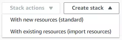
After you successfully issued our cloud formation scripts to Cloud Formation service, you can see the script progressing in the AWS console:
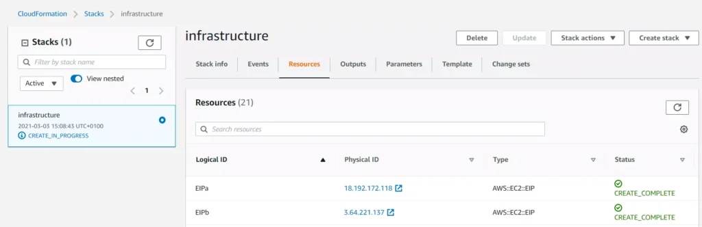
You may find Events and Resource tabs useful while you follow the resource creation procedure.
Once all infrastructure components are up and running, you’ll see your stack status marked as CREATE_COMPLETE :
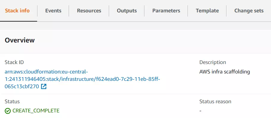
In case your infrastructure definition contained any errors, you will be able to see them in the Cloud Formation console events tab. The status reason column will contain an error message from Cloud Formation or a specific resource service. For example:

For more information on troubleshooting CloudFormation, visit the AWS documentation page .
Summary - cloud infrastructure as code in practice
If you’re reading this, congrats then! You’ve reached the end of this tutorial. We went through the basics of what Infrastructure as Code is, how it works and when to use it. Furthermore, we got a grasp of hands-on experience with Cloud Formation.
As a next step, we strongly encourage you to take a deep dive into AWS Cloud Formation documentation . It will help you adjust the infrastructure to your specific needs and make it even more bulletproof. Eventually, now with all of your infrastructure scripted, you can shout out loud: look ma, no hands!
Supplement - aka. Cloud Formation tips and tricks
When you’re done playing around with your CF Stacks, remember to delete them! Otherwise, AWS will charge you!
Cloud Formation does not warn you if your updated stack definition might cause infrastructure downtime (resource replacement needed). However, there are two ways to validate that before you deploy. The first one - manual - is to double-check specific resource documentation, especially if the updated property description contains Update requires : Replacement clause. See example for CidrBlock VPC property:
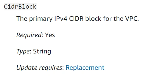
The second way is to use the Change Sets mechanism provided by Cloud Formation. This one would automatically validate the template and tell you how these changes might impact your infrastructure. See the docs .
Cloud Formation does not watch over your resources after they’re created. Therefore, if you make any manual modifications to the resource that is maintained by CF Stack, the stack itself won’t be updated. A situation where the actual infrastructure state is different from its definition (CF script) is called configuration drift. CF comes in handy and lets you see the actual drift for the stack in the console - see this .
If you create your own Cloud Formation script and looking for more examples, the CF registry might come in handy.

Personalized finance as a key driver leading Financial Services industry into the future
Personalization in finance is a process that has been steadily developing for the last decade. It’s the most crucial trend you can pay attention to as it captures the essence of what modern consumers want. Individual service and attention.
Personalized finance is a journey with the customer in focus. Getting closer to customers means meeting them where they are, understanding their individual goals, and providing advice they actually want need.
Technology has introduced a tremendous change in personal finance. While it hasn’t yet democratized traditional banking and finance the way it’s promised, it’s well on its way – transforming the way we budget, invest, save or borrow money today. As companies enter the post-pandemic world, they face a consumer landscape undergoing sudden and radical change. Customer expectations have been transformed to make “anywhere, anytime” the norm. Achieving personalization at scale will be definitely one of the biggest challenges for traditional institutions in the race to differentiate through a digital channel in the coming years.
Why personalization matters in Financial Services?
Personalized services shorten significantly the distance between a financial organization and its users, and are based on trust. The more we trust the product the more we are eager to share our personal data in order to receive a tailored, highly individualized service that maximizes value for customers. Trust is still the strongest word in banking. The 2020 Edelman Trust Barometer Spring Update: Special Report on Financial Services and the Covid-19 Pandemic reveals that the public’s trust in financial services has reached an all-time high of 65 percent amid the pandemic.
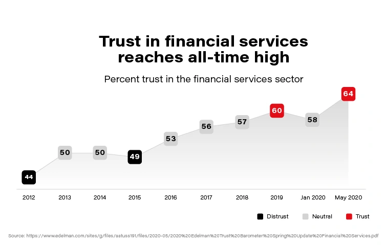
Now, when we associate the trust clients put i.e., into banks with the scale of daily operations (counted in millions), we easily conclude that there is an enormous opportunity in front of the financial sector to build highly personalized products and enable customers to realize their financial wellbeing potential.
With an increasing demand for more personalized experiences and focus on sustainability, Banks, Insurers, or Asset Management organizations are reaching the limits of where their current technology can take them with their business transformation initiatives. Therefore, it’s more critical than ever for Financial Institutions to turn towards Data and AI and get the most out of it - to meet these demands.
While reading different collaterals for the purpose of this article, we noticed an interesting paradox related to the financial domain. According to the variety of global innovation studies (i.e., Forbes Most Innovative Companies or The Global Innovation 1000 study), the Financial Services domain lacks innovation for nearly two decades. On the contrary, it has consistently been the most profitable sector in FORTUNE GLOBAL 500!
Data and AI for personalized finance
To make sure an organization stands out of the competition in an ever-changing financial environment and understands its customers better, it should radically change its approach to Data & AI utilization. Although traditional banks and financial enterprises differ by size, market dynamic, or type of services offering - there is a common set of requirements (attached below) worth taking into consideration when pivoting towards better personalization which can be achieved thanks to the advanced use of Data & AI within an enterprise:
- The Executive Board must believe that Data & AI will make a difference, and this commitment requires long-term investment/research.
- Organizations need to find a Champion that can lead a data/AI team, but at the same time be able to talk to the business stakeholders and articulate the benefits of the models *tools* being implemented.
- It’s necessary to spend time to create Data Strategy, determine a toolset, and figure out when to use Data vs. Analytics vs. AI. Without a strategy, an organization is flying blind and wastes precious time/resources *money*.
- Focus on what brings real value to the organization. Build a use case backlog that balances return on investment, time to market, innovation, and data availability. All of these are important and can help an organization determine where to start and why.
- Data Ethics, Privacy, and Governance are critical to not just the organization but its customers. Use their data inappropriately or violate their privacy even once, and you risk forever damaging the relationship (see recent case of Robinhood).
- Don't assume you can do it by yourself. Consider hiring, engage with a consulting partner, outsource - all of the above are likely required.
How does technology help achieve personalization at a large scale?
Commonwealth Bank of Australia and Royal Bank of Scotland are early adopters in the traditional banking ecosystem when it comes to personalized CX. These companies use advanced data analytics coupled with artificial intelligence to offer personalized experiences – technology that allowed them to determine and deliver ‘the next best conversation’ at scale saw a 30 to 40 percent increase in sales, back in 2017!
Personetics , a data-driven platform that uses AI to help banks issue personalized advice and insights to customers, has raised $75 million in funding from private equity firm Warburg Pincus. Founded out of Israel in 2010, Personetics offers technology that works inside financial institutions’ software. It aims to analyze customers’ financial transactions and behavior and deliver real-time tips and suggestions to improve their longer-term financial health.
In the latest report related to digitalization at Handelsbanken (one of the largest European banks with HQ in Sweden), we see practical examples of how technology played a vital role in building highly personal advisory services, which increased the customer value and realize the potential in their 35 million digital meetings per month by utilizing data and treating each customer as an individual.
Thinking about the scale and impact of the financial business, there was no better time in human history to maintain simultaneously hundreds of millions of interactions to deliver value per individual need. Advancements in automation, cloud computing, or machine intelligence technologies create new space for maximizing the power of data and give an enormous opportunity for traditional businesses to exponentially grow the quality of relationships and keeping up with customers.
It’s very hard to compete with an organization that is capable to save its clients precious time and deliver value which is a sum of trust + context + momentum in an engaging and simple to consume form.
Head of Digital at Bank of America, David Tyrie, shared an interesting viewpoint that refers to personalization challenges for the traditional banking ecosystem during discussion at the Digital Banking 2020 Conference:
Tailoring client experiences 1:1 to feel timely, relevant, and credible requires real-time decisioning of transactional, contextual, and behavioral data and an adoption of open platforms so that information can flow to trusted partners. “Closed-loop, data ecosystems” can help realize hyper-personalization at scale because they enable continuous learning to serve customized and contextual experiences, content, offers, recommendations, and insights.
This continuous learning component is vital as it helps big organizations like banks or insurers build more individualized interaction with their customers and learn their behavior along the way. We already see a growing post-pandemic trend to emulate everything that’s physical and build a digital representation of physical relationships to make sure the customer is at the heart of financial transformation.
Obstacles and opportunities for personalized finance
Personalization requires financial organizations to jump multiple levels when it comes to data maturity. In order to win the race for customer attention in 2021, companies should become not only a data organization from the ground up but to be flexible and fast with implementing new structures (incepting necessary cultural shift), systems and competencies (digital skills) that distinguish them from the old legacy times.
Even though increased focus on customers brings obvious benefits for both the organization and its clients, there are several significant challenges before financial enterprises can reap the great benefits from personalization. It’s worth making sure the organization is prepared and can handle some of the existing challenges:
- Data consists of a lot of unstructured content, which makes it difficult to interpret.
- Instead of considering data as an IT asset, the ownership of data should be moved to the business users, making data a key asset for decision making (it’s necessary to strengthen cooperation between business & tech, to tear down the product-silos).
- Restrictions of regulatory requirements and privacy concerns.
- Integrating customer data from multiple sources to create comprehensive profiles that are then used by predictive analytics tools to generate the most relevant recommendations and products might cause data quality issue due to third-party, publicly available data sources for which financial services companies can’t manage the reliability.
It seems unreal that the successful banks and financial industry organizations of tomorrow will be that far removed from those of today. Rather how customers interact with them will be different (digital customer interface). Financial services have become anything but personal. The relationship we have with our money is being completely reimagined for the digital world, same as how we go about building financial services is changing. We are sure this trend will not only grow but will be one of the key drivers in the financial services transformation .
Automating your enterprise infrastructure. Part 1: Introduction to cloud infrastructure as code (AWS Cloud Formation example)
This is the first article of the series that presents the path towards automated infrastructure deployment. In the first part, we focus on what Infrastructure as Code actually means, its main concepts and gently fill you in on AWS Cloud Formation. In the next part , we get some hands-on experience building and spinning up Enterprise Level Infrastructure as Code.
With a DevOps culture becoming a standard, we face automation everywhere. It is an essential part of our daily work to automate as much as possible. It simplifies and shortens our daily duties, which de facto leads to cost optimization. Moreover, respected developers, administrators, and enterprises rely on automation because it eliminates the probability of human error (which btw takes 2nd place when it comes to security breach causes ).
Additionally, our infrastructure gets more and more complicated as we evolve towards cloud-native and microservice architectures. That is why Infrastructure as code (IaC) came up. It’s an answer to the growing complexity of our systems.
What you’ll find in this article:
- We introduce you to the IaC concept - why do we need it?
- You’ll get familiar with the AWS tool for IaC: Cloud Formation
Why do we need to automate our enterprise infrastructure?
Let’s start with short stories. Close eyes and imagine this:
Sunny morning, your brand new startup service is booming. A surge of dollars flows into Your bank account. The developers have built nice microservice-oriented infrastructure, they’ve configured AWS infrastructure, all pretty shiny. Suddenly, You receive a phone call from someone who says that Amazon's cleaning lady slipped into one of the AWS data centers, fall on the computing rack, therefore the whole Availability Zone went down. Your service is down, users are unhappy.
You tell your developers to recreate the infrastructure in a different data center as fast as they can. Well, it turns out that it’s not possible as fast as you would wish. Last time, it took them a week to spin up the infrastructure, which consists of many parts… you’re doomed.
The story is an example of Disaster Recovery , or rather a lack of it. No one thought that anything might go wrong. But as Murphy’s law says: Anything that can go wrong will go wrong
The other story:
As a progressive developer, you’re learning bleeding-edge cloud technologies to keep up with changing requirements for your employer. You decided to use AWS. Following Michal's tutorial , you happily created your enterprise-level infrastructure. After a long day, you cheerfully lay down to bed. The horror begins when you enter your bank account at the end of the month. Seems that Amazon charged you, for the resources you didn’t delete.
You think these scenarios are unreal? Get to know these stories:
How do You avoid these scenarios? The simple answer to that is IaC.
Infrastructure as Code
Infrastructure as Code is a way to create a recipe for your infrastructure. Normally, a recipe consists of two parts: ingredients and directions/method on how to turn ingredients into the actual dish. IaC is similar, except the narration is a little bit different.
In practice, IaC says:
Keep your IaC scripts (infrastructure components definition) right next to your application code in the Git repository. Think about those definitions as simple text files containing descriptions of your infrastructure. In comparison to the metaphor above, IaC scripts (infrastructure components definitions) are ingredients .
IaC also tells you this:
Use or build tools that will seamlessly turn your IaC scripts into actual cloud resources. So translating that: use or build tools that will seamlessly turn your ingredients (IaC scripts) into a dish (cloud resources).
Nowadays, most IaC tools do the infrastructure provisioning for you and keep it idempotent . So, you just have to prepare the ingredients. Sounds cool, right?
Technically speaking, IaC states that similarly to the automated application build & deployment processes and tools, we should have processes and tools targeted for automated infrastructure deployment .
An important thing to note here is that the approach described above leans you towards GitOps and trunk-based CICD . It is not a coincidence that these concepts are often listed one next to the other. Eventually, this is a big part of what DevOps is all about.
Still not sure how IoC is beneficial to you? See this:
During the HacktOberFest conference, Michal has been setting up the infrastructure manually - live during his lecture. It took him around 30 minutes - even though Michal is an experienced player.
Using cloud formation scripts, the same infrastructure is up and running in ~5 minutes , besides it doesn’t mean that we have to continuously watch over the script being processed. We can just fire and forget, go, have a coffee for the remaining 4 minutes and 50 seconds.
To sum up:
30/5 = 6
Your infrastructure boots up 6 times faster and you have some extra free time. Eventually, it boils down only to the question if you can afford such a waste.
With that being said, we can clearly see that IaC is the foundation on top of which enterprises may implement:
- Highly Available systems
- Disaster recovery
- predictable deployments
- faster time to prod
- CI/CD
- Cost optimization
Note that IaC is just a guideline, and IaC tools are just tools that enable you to achieve the before-mentioned goals faster and better. No tool does the actual work for you.
Regardless of your specific needs, either you build enterprise infrastructure and want to have HA and DR or you just deploy your first application to the cloud and reduce the cost of it, IoC is beneficial for you.
Which IaC tool to use?
There are many IaC tool offerings on the market. Each claim to be the best one. Only to satisfy our AWS deployment automation, we can go with Terraform, AWS Cloud Formation, Ansible and many many more. Which one to use? There is no straight answer, as always in IT: it depends . We recommend doing a few PoC, try out various tools and afterward decide which one fits you best.
How do we do it? Cloud Formation
As aforementioned we need to transcribe our infrastructure into code. So, how do we do it?
First, we need a tool for that. So there it is, the missing piece of Enterprise level AWS Infrastructure - Cloud Formation . It’s an AWS native IaC tool commonly used to automate infrastructure deployment.
Simply put, AWS Cloud Formation scripts are simple text files containing definitions of AWS resources that your infrastructure utilizes (EC2, S3, VPC, etc.). In Cloud Formation these text files are called Templates.
Well… ok, actually Cloud Formation is a little bit more than that. It’s also an AWS service that accepts CF scripts and orchestrates AWS to spin up all of the resources you requested in the right order (simply, automates the clicking in the console). Besides, it gives you live insight into the requested resource status.
Cloud formation follows the notion of declarative infrastructure definitions. On the contrary to an imperative approach in which You say how to provision infrastructure, declaratively you just specify what is the expected result. The knowledge of how to spin up requested resources lies on the AWS side.
If You followed Michal Kapiczynski’s tutorials , the Cloud Formation scripts presented underneath are just all his heavy work, written down to ~500 lines of yml file that you can keep in the repository right next to your application.
Note: Further reading requires you to either see Michals articles before or basic knowledge of AWS.
Enterprise Level Infrastructure Overview
There are many expectations from Enterprise Level infrastructure. From our use case standpoint, we’ll guarantee High Availability, by deploying our infrastructure in two separate AWS Data Centers (Availability Zones) and provide data redundancy by database replication. The picture presented above visualizes the target state of our Enterprise Level Infrastructure.
TLDR; If You’re here just to see the finished Cloud Formation script, please go ahead and visit this GitHub repository .
We've decided to split up our infrastructure setup into two parts (scripts) called Templates . The first part includes AWS resources necessary to construct a network stack. The latter collects application-specific resources: virtual machines, database, and load balancer. In cloud formation nomenclature, each individual set of tightly related resources is called Stack .
Stack usually contains all resources necessary to implement planned functionality. It can consist of: VPC, Subnets, EC2 instances, Load Balancers, etc. This way, we can spin up and tear down all of the resources at once with just one click (or one CLI command).
Each Template can be parametrized. To achieve easy scaling capabilities and disaster recovery, we’ll introduce the Availability Zone parameter. It will allow us to deploy the infrastructure in any AWS data center all around the world just by changing the parameter value.
As you will see through the second part of the guide , Cloud Formation scripts include a few extra resources in comparison to what was originally shown in Michal’s Articles . That’s because AWS creates these resources automatically for you under the hood when you create the infrastructure manually. But since we’re doing the automation, we have to define these resources explicitly.
Sources:
- https://docs.aws.amazon.com/AWSCloudFormation/latest/UserGuide/gettingstarted.templatebasics.html
- https://martinfowler.com/bliki/InfrastructureAsCode.html
- https://docs.microsoft.com/en-us/azure/devops/learn/what-is-infrastructure-as-code