Monitoring your microservices on AWS with Terraform and Grafana - basic microservices architecture

Do you have an application in the AWS cloud? Do you have several microservices you would like to monitor? Or maybe you’re starting your new project and looking for some good-looking, well-designed infrastructure? Look no further - you are in the right place!
We’ve spent some time building and managing microservices and cloud-native infrastructure so we provide you with a guide covering the main challenges and proven solutions.
In this series, we describe the following topics:
- How to create a well-designed architecture with microservices and a cloud-config server?
- How to collect metrics and logs in a common dashboard?
- How to secure the entire stack?
Monitoring your microservices - assumptions
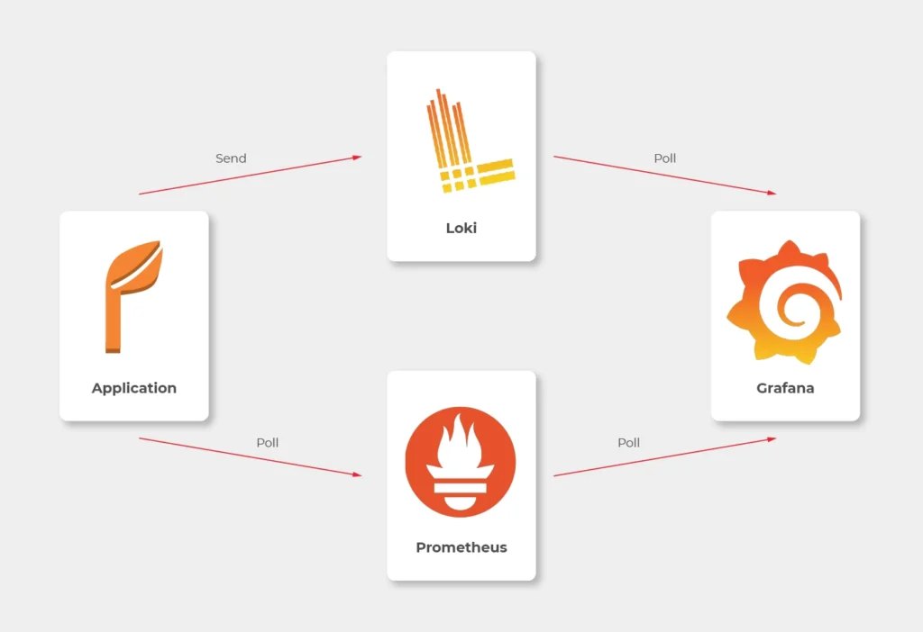
Choosing Grafana for such a project seems obvious, as the tool is powerful, fast, user-friendly, customizable, and easy to maintain. Grafana works perfectly with Prometheus and Loki. Prometheus is a metric sink that collects metrics from multiple sources and sends them to the target monitoring system. Loki does the very same operation for logs. Both collectors are designed to be integrated with Grafana.
See the diagram below to better understand our architecture:
Let’s analyze the diagram for a moment. On the top, there is a publicly visible hosted zone in Route 53, the DNS “entry” to our system, with 3 records: two application services available over the internet and an additional monitoring service for our internal purposes.
Below, there is a main VPC with two subnets: public and private. In the public one, we have load balancers only, and in the private one, there is an ECS cluster. In the cluster, we have few services running using Fargate: two with internet-available APIs, two for internal purposes, one Spring Cloud Config Server, and our monitoring stack: Loki, Prometheus, and Grafana. At the bottom of the diagram, you can also find a Service Discovery service (AWS CloudMap) that creates entries in Route 53, to enable communication inside our private subnet.
Of course, for readability reasons, we omit VPC configuration, services dependencies (RDS, Dynamo, etc.), CI/CD, and all other services around the core. You can follow this guide covering building AWS infrastructure.
To sum up our assumptions:
- We use an infra-as-a-code approach with Terraform
- There are few Internet-facing services and few for internal purposes in our private subnet
- Internet-facing services are exposed via load balancers in the public subnet
- We use the Fargate launch type for ECS tasks
- Some services can be scaled with ECS auto-scaling groups
- We use Service Discovery to redeploy and scale without manual change of IP’s, URL’s or target groups
- We don’t want to repeat ourselves so we use a Spring Cloud Config Server as a main source of configuration
- We use Grafana to see synchronized metrics and logs
- (what you cannot see on the diagram) We use encrypted communication everywhere - including communication between services in a private subnet
Basic AWS resources
In this article, we assume you have all basic resources already created and correctly configured: VPC, subnets, general security groups, network ACLs, network interfaces, etc. Therefore we’re going to focus on resources visible on the diagram above, crucial from a monitoring point of view.
Let’s create the first common resource:
resource "aws_service_discovery_private_dns_namespace" "namespace_for_environment" {
name = "internal"
vpc = var.vpc_id
}
This is the Service Discovery visible in the lower part of the diagram. We’re going to fill it in a moment.
By the way, above, you can see an example, how we’re going to present listings. You will need to adjust some variables for your needs (like var .vpc_id ). We strongly recommend using Terragrunt to manage dependencies between your Terraform modules, but it’s out of the scope of this paper.
Your services without monitoring
Internet-facing services
Now let’s start with the first application. We need something to monitor.
resource "aws_route53_record" "foo_entrypoint" {
zone_id = var.zone_environment_id
name = "foo"
type = "A"
set_identifier = "foo.example.com"
alias {
name = aws_lb.foo_ecs_alb.dns_name
zone_id = aws_lb.foo_ecs_alb.zone_id
evaluate_target_health = true
}
latency_routing_policy {
region = var.default_region
}
}
This is an entry for Route53 to access the internet-facing “foo” service. We’ll use it to validate a TLS certificate later.
resource "aws_lb" "foo_ecs_alb" {
name = "foo"
internal = false
load_balancer_type = "application"
security_groups = [
aws_security_group.alb_sg.id
]
subnets = var.vpc_public_subnet_ids
}
resource "aws_lb_target_group" "foo_target_group" {
name = "foo"
port = 8080
protocol = "HTTP"
target_type = "ip"
vpc_id = var.vpc_id
health_check {
port = 8080
protocol = "HTTP"
path = "/actuator/health"
matcher = "200"
}
depends_on = [
aws_lb.foo_ecs_alb
]
}
resource "aws_lb_listener" "foo_http_listener" {
load_balancer_arn = aws_lb.foo_ecs_alb.arn
port = "8080"
protocol = "HTTP"
default_action {
type = "forward"
target_group_arn = aws_lb_target_group.foo_target_group.arn
}
}
resource "aws_security_group" "alb_sg" {
name = "alb-sg"
description = "Inet to ALB"
vpc_id = var.vpc_id
ingress {
protocol = "tcp"
from_port = 8080
to_port = 8080
cidr_blocks = [
"0.0.0.0/0"
]
}
egress {
protocol = "-1"
from_port = 0
to_port = 0
cidr_blocks = [
"0.0.0.0/0"
]
}
}
OK, what do we have so far?
Besides the R53 entry, we’ve just created a load balancer, accepting traffic on 8080 port and transferring it to the target group called foo_target_group . We use a default Spring Boot " /actuator/health " health check endpoint (you need to have spring-boot-starter-actuator dependency in your pom) and a security group allowing ingress traffic to reach the load balancer and all egress traffic from the load balancer.
Now, let’s create the service.
resource "aws_ecr_repository" "foo_repository" {
name = "foo"
}
resource "aws_ecs_task_definition" "foo_ecs_task_definition" {
family = "foo"
network_mode = "awsvpc"
requires_compatibilities = ["FARGATE"]
cpu = "512"
memory = "1024"
execution_role_arn = var.ecs_execution_role_arn
container_definitions = <<TASK_DEFINITION
[
{
"cpu": 512,
"image": "${aws_ecr_repository.foo_repository.repository_url}:latest",
"memory": 1024,
"memoryReservation" : 512,
"name": "foo",
"networkMode": "awsvpc",
"essential": true,
"environment" : [
{ "name" : "SPRING_CLOUD_CONFIG_SERVER_URL", "value" : "configserver.internal" },
{ "name" : "APPLICATION_NAME", "value" : "foo" }
],
"portMappings": [
{
"containerPort": 8080,
"hostPort": 8080
}
]
}
]
TASK_DEFINITION
}
resource "aws_ecs_service" "foo_service" {
name = "foo"
cluster = var.ecs_cluster_id
task_definition = aws_ecs_task_definition.foo_ecs_task_definition.arn
desired_count = 2
launch_type = "FARGATE"
network_configuration {
subnets = var.vpc_private_subnet_ids
security_groups = [
aws_security_group.foo_lb_to_ecs.id,
aws_security_group.ecs_ecr_security_group.id,
aws_security_group.private_security_group.id
]
}
service_registries {
registry_arn = aws_service_discovery_service.foo_discovery_service.arn
}
load_balancer {
target_group_arn = aws_lb_target_group.foo_target_group.arn
container_name = "foo"
container_port = 8080
}
depends_on = [aws_lb.foo_ecs_alb]
}
You can find just three resources above, but a lot of configuration. The first one is easy - just an ECR for the image of your application. Then we have a task definition. Please pay attention to environment variables SPRING_CLOUD_CONFIG_SERVER_URL - this is an address of our config server inside our internal Service Discovery domain. The third one is an ECS service.
As you can see, it uses some magic of ECS Fargate - automatically registering new tasks in a Service Discovery ( service_registries section) and a load balancer ( load_balancer section). We just need to wait until the load balancer is created ( depends_on = [aws_lb.foo_ecs_alb] ). If you want to add some autoscaling, this is the right place to put it in. You’re also ready to push your application to the ECR if you already have one. We’re going to cover the application's important content later in this article. The ecs_execution_role_arn is just a standard role with AmazonECSTaskExecutionRolePolicy , allowed to be assumed by ECS and ecs-tasks.
Let’s discuss security groups now.
resource "aws_security_group" "foo_lb_to_ecs" {
name = "allow_lb_inbound_foo"
description = "Allow inbound Load Balancer calls"
vpc_id = var.vpc_id
ingress {
from_port = 8080
protocol = "tcp"
to_port = 8080
security_groups = [aws_security_group.foo_alb_sg.id]
}
}
resource "aws_security_group" "ecs_to_ecr" {
name = "allow_ecr_outbound"
description = "Allow outbound traffic for ECS task, to ECR/docker hub"
vpc_id = aws_vpc.main.id
egress {
from_port = 443
to_port = 443
protocol = "tcp"
cidr_blocks = ["0.0.0.0/0"]
}
egress {
from_port = 53
to_port = 53
protocol = "udp"
cidr_blocks = ["0.0.0.0/0"]
}
egress {
from_port = 53
to_port = 53
protocol = "tcp"
cidr_blocks = ["0.0.0.0/0"]
}
}
resource "aws_security_group" "private_inbound" {
name = "allow_inbound_within_sg"
description = "Allow inbound traffic inside this SG"
vpc_id = var.vpc_id
ingress {
from_port = 0
to_port = 0
protocol = "-1"
self = true
}
egress {
from_port = 0
to_port = 0
protocol = "-1"
self = true
}
}
As you can see, we use three groups - all needed. The first one allows the load balancer located in the public subnet to call the task inside the private subnet. The second one allows our ECS task to poll its image from the ECR. The last one allows our services inside the private subnet to talk to each other - such communication is allowed by default, only if you don’t attach any specific group (like the load balancer’s one), therefore we need to explicitly permit this communication.
There is just one piece needed to finish the “foo” service infrastructure - the service discovery service entry.
resource "aws_service_discovery_service" "foo_discovery_service" {
name = "foo"
description = "Discovery service name for foo"
dns_config {
namespace_id = aws_service_discovery_private_dns_namespace.namespace_for_environment.id
dns_records {
ttl = 100
type = "A"
}
}
}
It creates a “foo” record in an “internal” zone. So little and yet so much. The important thing here is - this is a multivalue record, which means it can cover 1+ entries - it provides basic, equal-weight autoscaling during normal operation but Prometheus can dig out from such a record each IP address separately to monitor all instances.
Now some good news - you can simply copy-paste the code of all resources with names prefixed with “foo_” and create “bar_” clones for the second, internet-facing service in the project. This is what we love Terraform for.
Backend services (private subnet)
This part is almost the same as the previous one, but we can simplify some elements.
resource "aws_ecr_repository" "backend_1_repository" {
name = "backend_1"
}
resource "aws_ecs_task_definition" "backend_1_ecs_task_definition" {
family = "backend_1"
network_mode = "awsvpc"
requires_compatibilities = ["FARGATE"]
cpu = "512"
memory = "1024"
execution_role_arn = var.ecs_execution_role_arn
container_definitions = <<TASK_DEFINITION
[
{
"cpu": 512,
"image": "${aws_ecr_repository.backend_1_repository.repository_url}:latest",
"memory": 1024,
"memoryReservation" : 512,
"name": "backend_1",
"networkMode": "awsvpc",
"essential": true,
"environment" : [
{ "name" : "_JAVA_OPTIONS", "value" : "-Xmx1024m -Xms512m" },
{ "name" : "SPRING_CLOUD_CONFIG_SERVER_URL", "value" : "configserver.internal" },
{ "name" : "APPLICATION_NAME", "value" : "backend_1" }
],
"portMappings": [
{
"containerPort": 8080,
"hostPort": 8080
}
]
}
]
TASK_DEFINITION
}
resource "aws_ecs_service" "backend_1_service" {
name = "backend_1"
cluster = var.ecs_cluster_id
task_definition = aws_ecs_task_definition.backend_1_ecs_task_definition.arn
desired_count = 1
launch_type = "FARGATE"
network_configuration {
subnets = var.vpc_private_subnet_ids
security_groups = [
aws_security_group.ecs_ecr_security_group.id,
aws_security_group.private_security_group.id
]
}
service_registries {
registry_arn = aws_service_discovery_service.backend_1_discovery_service.arn
}
}
resource "aws_service_discovery_service" "backend_1_discovery_service" {
name = "backend1"
description = "Discovery service name for backend 1"
dns_config {
namespace_id = aws_service_discovery_private_dns_namespace.namespace_for_environment.id
dns_records {
ttl = 100
type = "A"
}
}
}
As you can see, all resources related to the load balancer are gone. Now, you can copy the code about creating the backend_2 service.
So far, so good. We have created 4 services, but none will start without the config server yet.
Config server
The infrastructure for the config server is similar to the backed services described above. It simply needs to know all other services’ URLs. In the real-world scenario, the configuration may be stored in a git repository or in the DB, but it’s not needed for this article, so we’ve used a native config provider, with all config files stored locally.
We would like to dive into some code here, but there is not much in this module yet. To make it just working, we only need this piece of code:
@SpringBootApplication
@EnableConfigServer
public class CloudConfigServer {
public static void main(String[] arguments) {
run(CloudConfigServer.class, arguments);
}
}
and few dependencies.
<dependency>
<groupId>org.springframework.cloud</groupId>
<artifactId>spring-cloud-config-server</artifactId>
</dependency>
<dependency>
<groupId>org.springframework.boot</groupId>
<artifactId>spring-boot-starter-security</artifactId>
</dependency>
<dependency>
<groupId>org.springframework.boot</groupId>
<artifactId>spring-boot-starter-web</artifactId>
</dependency>
We also need some extra config in the pom.xml file.
<parent>
<groupId>org.springframework.boot</groupId>
<artifactId>spring-boot-starter-parent</artifactId>
<version>2.4.2</version>
</parent>
<dependencyManagement>
<dependencies>
<dependency>
<groupId>org.springframework.cloud</groupId>
<artifactId>spring-cloud-dependencies</artifactId>
<version>2020.0.1</version>
<type>pom</type>
<scope>import</scope>
</dependency>
</dependencies>
</dependencyManagement>
<build>
<plugins>
<plugin>
<groupId>org.springframework.boot</groupId>
<artifactId>spring-boot-maven-plugin</artifactId>
</plugin>
</plugins>
</build>
That’s basically it - you have your own config server. Now, let’s put some config inside. The Structure of the server is as follows.
config_server/
├─ src/
│ ├─ main/
│ ├─ java/
│ ├─ com/
│ ├─ example/
│ ├─ CloudConfigServer.java
│ ├─ resources/
│ ├─ application.yml (1)
│ ├─ configforclients/
│ ├─ application.yml (2)
As there are two files called application.yml we’ve added numbers (1), (2) at the end of lines to distinguish them. So the application.yml (1) file is there to configure the config server itself. Its content is as follows:
server:
port: 8888
spring:
application:
name: spring-cloud-config-server
profiles:
include: native
cloud:
config:
server:
native:
searchLocations: classpath:/configforclients
management:
endpoints:
web:
exposure:
include: health
With the “native” configuration, the entire classpath:/ and classpath:/config are taken as a configuration for remote clients. Therefore, we need this line:
spring.cloud.config.server.native.searchLocations: classpath:/configforclients to distinguish the configuration for the config server itself and for the clients. The client’s configuration is as follows:
address:
foo: ${FOO_URL:http://localhost:8080}
bar: ${BAR_URL:http://localhost:8081}
backend:
one: ${BACKEND_1_URL:http://localhost:8082}
two: ${BACKEND_2_URL:http://localhost:8083}
management:
endpoints:
web:
exposure:
include:health
spring:
jackson:
default-property-inclusion: non_empty
time-zone: Europe/Berlin
As you can see, all service discovery addresses are here, so they can be used by all clients. We also have some common configurations, like Jackson-related, and one important for the infra - to expose health checks for load balancers.
If you use Spring Boot Security (I hope you do), you can disable it here - it will make accessing the config server simpler, and, as it’s located in the private network and we’re going to encrypt all endpoints in a moment - you don’t need it. Here is an additional file to disable it.
@Configuration
@EnableWebSecurity
public class WebSecurityConfig extends WebSecurityConfigurerAdapter {
@Override
public void configure(WebSecurity web) throws Exception {
web.ignoring().antMatchers("/**");
getHttp().csrf().disable();
}
}
Yes, we know, it's strange to use @EnableWebSecurity to disable web security, but it’s how it works. Now, let’s configure clients to read those configurations.
Config clients
First of all, we need two dependencies.
<dependency>
<groupId>org.springframework.cloud</groupId>
<artifactId>spring-cloud-starter-bootstrap</artifactId>
</dependency>
<dependency>
<groupId>org.springframework.cloud</groupId>
<artifactId>spring-cloud-starter-config</artifactId>
</dependency>
We assume you have all Spring-Boot related dependencies already in place.
As you can see, we need to use bootstrap, so instead of the application.yml file, we’re going to use bootstrap.yml(which is responsible for loading configuration from external sources):
main:
banner-mode: 'off'
cloud:
config:
uri: ${SPRING_CLOUD_CONFIG_SERVER:http://localhost:8888}
There are only two elements here. We use the first one just to show you that some parameters simply cannot be set using the config server. In this example, main.banner-mode is being read before accessing the config server, so if you want to disable the banner (or change it) - you need to do it in each application separately. The second property - cloud.config.uri - is obviously a pointer to the config server. As you can see, we use a fallback value to be able to run everything both in AWS and local machines.
Now, with this configuration, you can really start every service and make sure that everything works as expected.
Monitoring your microservices - conclusion
That was the easy part. Now you have a working application, exposed and configurable. We hope you can tweak and adjust it for your own needs. In the next part we’ll dive into a monitoring topic.

Grape Up guides enterprises on their data-driven transformation journey
Ready to ship? Let's talk.
Check related articles
Read our blog and stay informed about the industry's latest trends and solutions.
Monitoring your microservices on AWS with Terraform and Grafana - monitoring
Welcome back to the series. We hope you’ve enjoyed the previous part and you’re back to learn the key points. Today we’re going to show you how to monitor the application.
Monitoring
We would like to have logs and metrics in a single place. Let’s imagine you see something strange on your diagrams, mark it with your mouse, and immediately have proper log entries from this particular timeframe and this particular machine displayed below. Now, let’s make it real.
Some basics first. There is a huge difference between the way Prometheus and Loki get the data. Both of them are being called by Grafana to poll data, but Prometheus also actively calls the application to poll metrics. Loki, instead, just listens, so it needs some extra mechanism to receive logs from applications.
In most sources over the Internet, you’ll find that the best way to send logs to Loki is to use Promtail. This is a small tool, developed by Loki’s authors, which reads log files and sends them entry by entry to remote Loki’s endpoint. But it’s not perfect. Sending multiline logs is still in a bad shape (state for February 2021), some config is really designed to work with Kubernetes only and at the end of the day, this is one more additional application you would need to run inside your Docker image, which can get a little bit dirty. Instead, we propose to use a loki4j logback appender (https://github.com/loki4j). This is a zero-dependency Java library designed to send logs directly from your application.
There is one more Java library needed - Micrometer . We’re going to use it to collect metrics of the application.
So, the proper diagram should look like this.
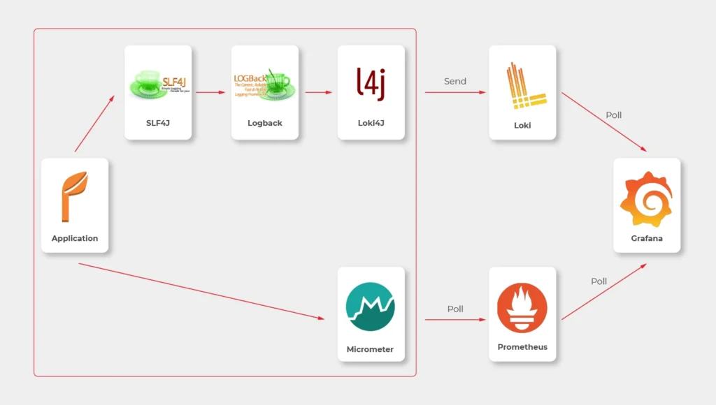
Which means, we need to build or configure the following pieces:
- slf4j (default configuration is enough)
- Logback
- Loki4j
- Loki
- Micrometer
- Prometheus
- Grafana
Micrometer
Let’s start with metrics first.
There are just three things to do on the application side.
The first one is to add a dependency to the Micrometer with Prometheus integration (registry).
<dependency>
<groupId>io.micrometer</groupId>
<artifactId>micrometer-registry-prometheus</artifactId>
</dependency>
Now, we have a new endpoint exposable from Spring Boot Actuator, so we need to enable it.
management:
endpoints:
web:
exposure:
include: prometheus,health
This is a piece of configuration to add. Make sure you include prometheus in both config server and config clients’ configuration. If you have some Web Security configured, make sure to enable full access to /actuator/health and /actuator/prometheus endpoint.
Now we would like to distinguish applications in our metrics, so we have to add a custom tag in all applications. We propose to add this piece of code as a Java library and import it with Maven.
@Configuration
public class MetricsConfig {
@Bean
MeterRegistryCustomizer<MeterRegistry> configurer(@Value("${spring.application.name}") String applicationName) {
return (registry) -> registry.config().commonTags("application", applicationName);
}
}
Make sure you have spring.application.name configured in all bootstrap.yml files in config clients and application.yml in the config server.
Prometheus
The next step is to use a brand new /actuator/prometheus endpoint to read metrics in Prometheus.
The ECS configuration is similar to backend services. The image you need to push to your ECR should look like that.
FROM prom/prometheus
COPY prometheus.yml .
ENTRYPOINT prometheus --config.file=prometheus.yml
EXPOSE 9090
As Prometheus doesn’t support HTTPS endpoints, it’s just a temporary solution, and we’ll change it later.
The prometheus.yml file contains such a configuration.
scrape_configs:
- job_name: 'cloud-config-server'
metrics_path: '/actuator/prometheus'
scrape_interval: 5s
dns_sd_configs:
- names:
- '$cloud_config_server_url'
type: 'A'
port: 8888
- job_name: 'foo'
metrics_path: '/actuator/prometheus'
scrape_interval: 5s
dns_sd_configs:
- names:
- '$foo_url
type: 'A'
port: 8080
- job_name: bar
metrics_path: '/actuator/prometheus'
scrape_interval: 5s
dns_sd_configs:
- names:
- '$bar_url
type: 'A'
port: 8080
- job_name: 'backend_1'
metrics_path: '/actuator/prometheus'
scrape_interval: 5s
dns_sd_configs:
- names:
- '$backend_1_url
type: 'A'
port: 8080
- job_name: 'backend_2'
metrics_path: '/actuator/prometheus'
scrape_interval: 5s
dns_sd_configs:
- names:
- '$backend_2_url
type: 'A'
port: 8080
Let’s analyse the first job as an example.
We would like to call '$cloud_config_server_url' url with '/actuator/prometheus' relative path on a port 8080 . As we’ve used dns_sd_configs and type: 'A', the Prometheus can handle multivalue DNS answers from the Service Discovery, to analyze all tasks in each service. Please make sure you replace all ' $x' variables in the file with proper URLs from the Service Discovery.
The Prometheus isn’t exposed to the public load balancer, so you cannot verify your success so far. You can expose it temporarily or wait for Grafana.
Logback and Loki4j
If you use the Spring Boot, you probably already have spring-boot-starter-logging
library included. Therefore, you use logback as the default slf4j integration. Our job now is to configure it to send logs to Loki. Let’s start with the dependency:
<dependency>
<groupId>com.github.loki4j</groupId>
<artifactId>loki-logback-appender</artifactId>
<version>1.1.0</version>
</dependency>
Now let’s configure it. The first file is called logback-spring.xml and located in the config server next to the application.yml (1) file.
<?xml version="1.0" encoding="UTF-8"?>
<configuration>
<property name="LOG_PATTERN" value="%d{yyyy-MM-dd HH:mm:ss.SSS} %-5level [%thread] %logger - %msg%n"/>
<appender name="Console" class="ch.qos.logback.core.ConsoleAppender">
<encoder>
<pattern>${LOG_PATTERN}</pattern>
</encoder>
</appender>
<springProfile name="aws">
<appender name="Loki" class="com.github.loki4j.logback.Loki4jAppender">
<http>
<url>${LOKI_URL}/loki/api/v1/push</url>
</http>
<format class="com.github.loki4j.logback.ProtobufEncoder">
<label>
<pattern>application=spring-cloud-config-server,instance=${INSTANCE},level=%level</pattern>
</label>
<message>
<pattern>${LOG_PATTERN}</pattern>
</message>
<sortByTime>true</sortByTime>
</format>
</appender>
</springProfile>
<root level="INFO">
<appender-ref ref="Console"/>
<springProfile name="aws">
<appender-ref ref="Loki"/>
</springProfile>
</root>
</configuration>
What do we have here? There are two appenders with the common pattern, and one root logger. So we start with pattern configuration <property name="LOG_PATTERN" value="%d{yyyy-MM-dd HH:mm:ss.SSS} %-5level [%thread] %logger - %msg%n"/> . Of course you can configure it, as you want.
Then, the standard console appender. As you can see, it uses the LOG_PATTERN .
Then you can see the com.github.loki4j.logback.Loki4jAppender appender. This way the library is being used. We’ve used < springProfile name="aws" > profile filter to enable it only in the AWS infrastructure and disable locally. We use the same when using the appender with appender-ref ref="Loki" . Please note the label pattern, used here to label each log with custom tags (application, instance, level). Another important part here is Loki’s URL. We need to provide it as an environment variable for the ECS task. To do that, you need to add one more line to your aws_ecs_task_definition configuration in terraform.
"environment" : [
...
{ "name" : "LOKI_URL", "value" : "loki.internal" }
],
As you can see, we defined “loki.internal” URL and we’re going to create it in a minute.
There are few issues with logback configuration for the config clients.
First of all, you need to provide the same LOKI_URL environment variable to each client, because you need Loki before reading config from the config server.
Now, let’s put another logback-spring.xml file in the config server next to the applic ation.yml (2) file.
<?xml version="1.0" encoding="UTF-8"?>
<configuration>
<property name="LOG_PATTERN" value="%d{yyyy-MM-dd HH:mm:ss.SSS} %-5level [%thread] %logger - %msg%n"/>
<springProperty scope="context" name="APPLICATION_NAME" source="spring.application.name"/>
<appender name="Console" class="ch.qos.logback.core.ConsoleAppender">
<encoder>
<pattern>\${LOG_PATTERN}</pattern>
</encoder>
</appender>
<springProfile name="aws">
<appender name="Loki" class="com.github.loki4j.logback.Loki4jAppender">
<http>
<requestTimeoutMs>15000</requestTimeoutMs>
<url>\${LOKI_URL}/loki/api/v1/push</url>
</http>
<format class="com.github.loki4j.logback.ProtobufEncoder">
<label>
<pattern>application=\${APPLICATION_NAME},instance=\${INSTANCE},level=%level</pattern>
</label>
<message>
<pattern>\${LOG_PATTERN}</pattern>
</message>
<sortByTime>true</sortByTime>
</format>
</appender>
</springProfile>
<root level="INFO">
<appender-ref ref="Console"/>
<springProfile name="aws"><appender-ref ref="Loki"/></springProfile>
</root>
</configuration>
The first change to notice are slashes before environment variables (eg. \${LOG_PATTERN } ). We need it to tell the config server not to resolve variables on it’s side (because it’s impossible). The next difference is a new variable <springProperty scope="context" name="APPLICATION_NAME" source="spring.application.name"/> . with this line and spring.application.name in all your applications each log will be tagged with a different name. There is also a trick with the ${INSTANCE} variable. As Prometheus uses IP address + port as an instance identifier and we want to use the same here, we need to provide this data to each instance separately.
So your Dockerfile files for your applications should have something like that.
FROM openjdk:15.0.1-slim
COPY /target/foo-0.0.1-SNAPSHOT.jar .
ENTRYPOINT INSTANCE=$(hostname -i):8080 java -jar foo-0.0.1-SNAPSHOT.jar
EXPOSE 8080
Also, to make it working, you are supposed to tell your clients to use this configuration. Just add this to bootstrap.yml files in all you config clients.
logging:
config: ${SPRING_CLOUD_CONFIG_SERVER:http://localhost:8888}/application/default/main/logback-spring.xml
spring:
application:
name: foo
That’s it, let’s move to the next part.
Loki
Creating Loki is very similar to Prometheus. Your dockerfile is as follows.
FROM grafana/loki
COPY loki.yml .
ENTRYPOINT loki --config.file=loki.yml
EXPOSE 3100
The good news is, you don’t need to set any URLs here - Loki doesn’t send any data. It just listens.
As a configuration, you can use a file from https://grafana.com/docs/loki/latest/configuration/examples/ . We’re going to adjust it later, but it’s enough for now.
Grafana
Now, we’re ready to put things together.
In the ECS configuration, you can remove service discovery stuff and add a load balancer, because Grafana will be visible over the internet. Please remember, it’s exposed at port 3000 by default.
Your Grafana Dockerfile should be like that.
FROM grafana/grafana
COPY loki_datasource.yml /etc/grafana/provisioning/datasources/
COPY prometheus_datasource.yml /etc/grafana/provisioning/datasources/
COPY dashboad.yml /etc/grafana/provisioning/dashboards/
COPY *.json /etc/grafana/provisioning/dashboards/
ENTRYPOINT [ "/run.sh" ]
EXPOSE 3000
Let’s check configuration files now.
loki_datasource.yml:
apiVersion: 1
datasources:
- name: Loki
type: loki
access: proxy
url: http://$loki_url:3100
jsonData:
maxLines: 1000
I believe the file content is quite obvious (we'll return here later).
prometheus_datasource.yml:
apiVersion: 1
datasources:
- name: prometheus
type: prometheus
access: proxy
orgId: 1
url: https://$prometheus_url:9090
isDefault: true
version: 1
editable: false
dashboard.yml:
apiVersion: 1
providers:
- name: 'Default'
folder: 'Services'
options:
path: /etc/grafana/provisioning/dashboards
With this file, you tell Grafana to install all json files from /etc/grafana/provisioning/dashboards directory as dashboards.
The last leg is to create some dashboards. You can, for example, download a dashboard from https://grafana.com/grafana/dashboards/10280 and replace ${DS_PROMETHEUS} datasource with your name “prometheus”.
Our aim was to create a dashboard with metrics and logs at the same screen. You can play with dashboards as you want, but take this as an example.
{
"annotations": {
"list": [
{
"builtIn": 1,
"datasource": "-- Grafana --",
"enable": true,
"hide": true,
"iconColor": "rgba(0, 211, 255, 1)",
"name": "Annotations & Alerts",
"type": "dashboard"
}
]
},
"editable": true,
"gnetId": null,
"graphTooltip": 0,
"id": 2,
"iteration": 1613558886505,
"links": [],
"panels": [
{
"aliasColors": {},
"bars": false,
"dashLength": 10,
"dashes": false,
"datasource": null,
"fieldConfig": {
"defaults": {
"custom": {}
},
"overrides": []
},
"fill": 1,
"fillGradient": 0,
"gridPos": {
"h": 8,
"w": 24,
"x": 0,
"y": 0
},
"hiddenSeries": false,
"id": 4,
"legend": {
"avg": false,
"current": false,
"max": false,
"min": false,
"show": true,
"total": false,
"values": false
},
"lines": true,
"linewidth": 1,
"nullPointMode": "null",
"options": {
"alertThreshold": true
},
"percentage": false,
"pluginVersion": "7.4.1",
"pointradius": 2,
"points": false,
"renderer": "flot",
"seriesOverrides": [],
"spaceLength": 10,
"stack": false,
"steppedLine": false,
"targets": [
{
"expr": "system_load_average_1m{instance=~\"$instance\", application=\"$application\"}",
"interval": "",
"legendFormat": "",
"refId": "A"
}
],
"thresholds": [],
"timeRegions": [],
"title": "Panel Title",
"tooltip": {
"shared": true,
"sort": 0,
"value_type": "individual"
},
"type": "graph",
"xaxis": {
"buckets": null,
"mode": "time",
"name": null,
"show": true,
"values": []
},
"yaxes": [
{
"format": "short",
"label": null,
"logBase": 1,
"max": null,
"min": null,
"show": true
},
{
"format": "short",
"label": null,
"logBase": 1,
"max": null,
"min": null,
"show": true
}
],
"yaxis": {
"align": false,
"alignLevel": null
}
},
{
"datasource": "Loki",
"fieldConfig": {
"defaults": {
"custom": {}
},
"overrides": []
},
"gridPos": {
"h": 33,
"w": 24,
"x": 0,
"y": 8
},
"id": 2,
"options": {
"showLabels": false,
"showTime": false,
"sortOrder": "Ascending",
"wrapLogMessage": true
},
"pluginVersion": "7.3.7",
"targets": [
{
"expr": "{application=\"$application\", instance=~\"$instance\", level=~\"$level\"}",
"hide": false,
"legendFormat": "",
"refId": "A"
}
],
"timeFrom": null,
"timeShift": null,
"title": "Logs",
"type": "logs"
}
],
"schemaVersion": 27,
"style": "dark",
"tags": [],
"templating": {
"list": [
{
"allValue": null,
"current": {
"selected": false,
"text": "foo",
"value": "foo"
},
"datasource": "prometheus",
"definition": "label_values(application)",
"description": null,
"error": null,
"hide": 0,
"includeAll": false,
"label": "Application",
"multi": false,
"name": "application",
"options": [],
"query": {
"query": "label_values(application)",
"refId": "prometheus-application-Variable-Query"
},
"refresh": 2,
"regex": "",
"skipUrlSync": false,
"sort": 0,
"tagValuesQuery": "",
"tags": [],
"tagsQuery": "",
"type": "query",
"useTags": false
},
{
"allValue": null,
"current": {
"selected": false,
"text": "All",
"value": "$__all"
},
"datasource": "prometheus",
"definition": "label_values(jvm_classes_loaded_classes{application=\"$application\"}, instance)",
"description": null,
"error": null,
"hide": 0,
"includeAll": true,
"label": "Instance",
"multi": false,
"name": "instance",
"options": [],
"query": {
"query": "label_values(jvm_classes_loaded_classes{application=\"$application\"}, instance)",
"refId": "prometheus-instance-Variable-Query"
},
"refresh": 2,
"regex": "",
"skipUrlSync": false,
"sort": 0,
"tagValuesQuery": "",
"tags": [],
"tagsQuery": "",
"type": "query",
"useTags": false
},
{
"allValue": null,
"current": {
"selected": false,
"text": [
"All"
],
"value": [
"$__all"
]
},
"datasource": "Loki",
"definition": "label_values(level)",
"description": null,
"error": null,
"hide": 0,
"includeAll": true,
"label": "Level",
"multi": true,
"name": "level",
"options": [
{
"selected": true,
"text": "All",
"value": "$__all"
},
{
"selected": false,
"text": "ERROR",
"value": "ERROR"
},
{
"selected": false,
"text": "INFO",
"value": "INFO"
},
{
"selected": false,
"text": "WARN",
"value": "WARN"
}
],
"query": "label_values(level)",
"refresh": 0,
"regex": "",
"skipUrlSync": false,
"sort": 0,
"tagValuesQuery": "",
"tags": [],
"tagsQuery": "",
"type": "query",
"useTags": false
}
]
},
"time": {
"from": "now-24h",
"to": "now"
},
"timepicker": {},
"timezone": "",
"title": "Logs",
"uid": "66Yn-8YMz",
"version": 1
}
We don’t recommend playing with such files manually when you can use a very convenient UI and export a json file later on. Anyway, the listing above is a good place to start. Please note the following elements:
In variable’s definitions, we use Prometheus only, because Loki doesn’t expose any metric so you cannot filter one variable (instance) when another one (application) is selected.
Because we would like to sometimes see all instances or log levels together, we need to query data like here: {application=\"$application\", instance=~\"$instance\", level=~\"$level \"}" . The important element is a tilde in instance=~\"$instance\" and level=~\"$level\" , which allows us to use multiple values.
Conclusion
Congratulation! You have your application monitored. We hope you like it! But please remember - it’s not production-ready yet! In the last part, we’re going to cover a security issue - add encryption at transit to all components.
Serverless architecture with AWS Cloud Development Kit (CDK)
The IT world revolves around servers - we set up, manage, and scale them, we communicate with them, deploy software onto them, and restrict access to them. In the end, it is difficult to imagine our lives without them. However, in this “serverfull” world, an idea of serverless architecture arose. A relatively new approach to building applications without direct access to the servers required to run them. Does it mean that the servers are obsolete, and that we no longer should use them? In this article, we will explore what it means to build a serverless application, how it compares to the well-known microservice design, what are the pros and cons of this new method and how to use the AWS Cloud Development Kit framework to achieve that.
Background
There was a time when the world was inhabited by creatures known as “monolith applications”. Those beings were enormous, tightly coupled, difficult to manage, and highly resource-consuming, which made the life of tech people a nightmare.
Out of that nightmare, a microservice architecture era arose, which was like a new day for software development. Microservices are small independent processes communicating with each other through their APIs. Each microservice can be developed in a different programming language, best suited for its job, providing a great deal of flexibility for developers. Although the distributed nature of microservices increased the overall architectural complexity of the systems, it also provided the biggest benefit of the new approach, namely scalability, coming from the possibility to scale each microservice individually based on its resource demands.
The microservice era was a life changer for the IT industry. Developers could focus on the design and development of small modular components instead of struggling with enormous black box monoliths. Managers enjoyed improvements in efficiency. However, microservice architecture still posed a huge challenge in the areas of deployment and infrastructure management for distributed systems. What is more, there were scenarios when it was not as cost-effective as it could be. That is how the software architecture underwent another major shift. This time towards the serverless architecture epoch.
What is serverless architecture?
Serverless, a bit paradoxically, does not mean that there are no servers. Both server hardware and server processes are present, exactly as in any other software architecture. The difference is that the organization running a serverless application is not owning and managing those servers. Instead, they make use of third-party Backend as a Service (BaaS) and/or Function as a Service platform.
- Backend as a Service (BaaS) is a cloud service model where the delivery of services responsible for server-side logic is delegated to cloud providers. This often includes services such as: database management, cloud storage, user authentication, push notifications, hosting, etc. In this approach, client applications, instead of talking to their dedicated servers, directly operate on those cloud services.

- Function as a Service (FaaS) is a way of executing our code in stateless, ephemeral computing environments fully managed by third-party providers without thinking about the underlying servers. We simply upload our code, and the FaaS platform is responsible for running it. Our functions can then be triggered by events such as HTTP(S) requests, schedulers, or calls from other cloud services. One of the most popular implementations of FaaS is the AWS Lambda service, but each cloud provider has its corresponding options.

In this article, we will explore the combination of both BaaS and FaaS approaches as most enterprise-level solutions combine both of them into a fully functioning system.
Note: This article is often referencing services provided by AWS . However, it is important to note that the serverless architecture approach is not cloud-provider-specific and most of the services mentioned as part of the AWS platform have their equivalents in other cloud platforms.
Serverless architecture design
We know a bit of theory, so let us look now at a practical example. The figure 1 presents an architecture diagram of a user management system created with the serverless approach.

The system utilizes Amazon Cognito for user authentication and authorization, ensuring that only authorized parties access our API. Then we have the API Gateway, which deals with all the routing, requests throttling, DDOS protection etc. API Gateway also allows us to implement custom authorizers if we can’t or don’t want to use Amazon Cognito. The business logic layer consists of Lambda Functions. If you are used to the microservice approach, you can think of each lambda as a separate set of a controller endpoint and service method, handling a specific type of request. Lambdas further communicate with other services such as databases, caches, config servers, queues, notification services, or whatever else our application may require.
The presented diagram demonstrates a relatively simple API design. However, it is good to bear in mind that the serverless approach is not limited to APIs. It is also perfect for more complex solutions such as data processing, batch processing, event ingestion systems, etc.
Serverless vs Microservices
Microservice-oriented architecture broke down the long-lasting realm of monolith systems through the division of applications into small, loosely coupled services that could be developed, deployed, and maintained independently. Those services had distinct responsibilities and could communicate with each other through APIs, constituting together a much larger and complex system. Up till this point, serverless does not differ much from the microservice approach. It also divides a system into smaller, independent components, but instead of services, we usually talk about functions.
So, what’s the difference? The microservices are standalone applications, usually packaged as lightweight containers and run on physical servers (commonly in the cloud), which you can access, manage and scale if needed. Those containers need to be supervised (orchestrated) with the use of tools such as Kubernetes . So speaking simply, you divide your application into smaller independent parts, package them as containers, deploy on servers, and orchestrate their lifecycle.
In comparison, when it comes to serverless functions, you only write your function code, upload it to the FaaS provider platform, and the cloud provider handles its packaging, deployment, execution, and scaling without showing you (or giving you access to) physical resources required to run it. What is more, when you deploy microservices, they are always active, even when they do not perform any processing, on the servers provisioned to them. Therefore, you need to pay for required host servers on a daily or monthly basis, in contrast to the serverless functions, which are only brought to life for their time of execution, so if there are no requests they do not use any resources.

Pros & cons of serverless computing
Pros:
- Pricing - Serverless works in a pay-as-you-go manner, which means that you only pay for those resources which you actually use, with no payment for idle time of the servers and no in-front dedication. This is especially beneficial for applications with infrequent traffic or startup organizations.
- Operational costs and complexity - The management of your infrastructure is delegated almost entirely to the cloud provider. This frees up your team allocation, decreases the probability of error on your side, and automates downtime handling leading to the overall increase in the availability of your system and the decrease in operational costs.
- Scalability by design - Serverless applications are scalable by nature. The cloud provider handles scaling up and down of resources automatically based on the traffic.
Cons:
- It is a much less mature approach than microservices which means a lot of unknowns and spaces for bad design decisions exist.
- Architectural complexity - Serverless functions are much more granular than microservices, and that can lead to higher architectural complexity, where instead of managing a dozen of microservices, you need to handle hundreds of lambda functions.
- Cloud provider specific solutions - With microservices packaged as containers, it didn’t matter which cloud provider you used. That is not the case for serverless applications which are tightly bound to the services provided by the cloud platform.
- Services limitations - some Faas and BaaS services have limitations such as a maximum number of concurrent requests, memory, timeouts, etc. which are often customizable but only to a certain point (e.g., default AWS Lambda execution quota equals 1000).
- Cold starts - Serverless applications can introduce response delays when a new instance handles its first request because it needs to boot up, copy application code, etc. before it can run the logic.
How much does it really cost?
One of the main advantages of the serverless design is its pay-as-you-go model, which can greatly decrease the overall costs of your system. However, does it always lead to lesser expenses? For this consideration, let us look at the pricing of some of the most common AWS services.
Service Price API Gateway 3.50$ per 1M requests (REST Api) Lambda 0.20$ per 1M request SQS First 1M free, then 0.40& per 1M requests
Those prices seem low, and in many cases, they will lead to very cheap operational costs of running serverless applications. Having that said, there are some scenarios where serverless can get much more expensive than other architectures. Let us consider a system that handles 5 mln requests per hour. Having it designed as a serverless architecture will lead to the cost of API Gateway only equal to:
$3.50 * 5 * 24 * 30 = $12,600/month
In this scenario, it could be more efficient to have an hourly rate-priced load balancer and a couple of virtual machines running. Then again, we would have to take into consideration the operational cost of setting up and managing the load balancer and VMs. As you can see, it all depends on the specific use case and your organization. You can read more about this scenario in this article .
AWS Cloud Development Kit
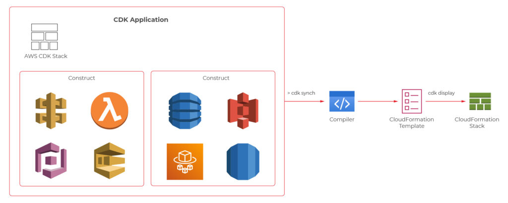
At this point, we know quite a lot about serverless computing, so now, let’s take a look at how we can create our serverless applications. First of all, we can always do it manually through the cloud provider’s console or CLI. It may be a valuable educational experience, but we wouldn’t recommend it for real-life systems. Another well-known solution is using Infrastructure as a Code (IaaS), such as AWS Cloud Formation service . However, in 2019 AWS introduced another possibility which is AWS Cloud Development Kit (CDK).
AWS CDK is an open-source software development framework which lets you define your architectures using traditional programming languages such as Java, Python, Javascript, Typescript, and C#. It provides you with high-level pre-configured components called constructs which you can use and further extend in order to build your infrastructures faster than ever. AWS CDK utilizes Cloud Formation behind the scenes to provision your resources in a safe and repeatable manner.
We will now take a look at the CDK definitions of a couple of components from the user management system, which the architecture diagram was presented before.
Main stack definition
export class UserManagerServerlessStack extends cdk.Stack {
private static readonly API_ID = 'UserManagerApi';
constructor(scope: cdk.Construct, id: string, props?: cdk.StackProps) {
super(scope, id, props);
const cognitoConstruct = new CognitoConstruct(this)
const usersDynamoDbTable = new UsersDynamoDbTable(this);
const lambdaConstruct = new LambdaConstruct(this, usersDynamoDbTable);
new ApiGatewayConstruct(this, cognitoConstruct.userPoolArn, lambdaConstruct);
}
}
API gateway
export class ApiGatewayConstruct extends Construct {
public static readonly ID = 'UserManagerApiGateway';
constructor(scope: Construct, cognitoUserPoolArn: string, lambdas: LambdaConstruct) {
super(scope, ApiGatewayConstruct.ID);
const api = new RestApi(this, ApiGatewayConstruct.ID, {
restApiName: 'User Manager API'
})
const authorizer = new CfnAuthorizer(this, 'cfnAuth', {
restApiId: api.restApiId,
name: 'UserManagerApiAuthorizer',
type: 'COGNITO_USER_POOLS',
identitySource: 'method.request.header.Authorization',
providerArns: [cognitoUserPoolArn],
})
const authorizationParams = {
authorizationType: AuthorizationType.COGNITO,
authorizer: {
authorizerId: authorizer.ref
},
authorizationScopes: [`${CognitoConstruct.USER_POOL_RESOURCE_SERVER_ID}/user-manager-client`]
};
const usersResource = api.root.addResource('users');
usersResource.addMethod('POST', new LambdaIntegration(lambdas.createUserLambda), authorizationParams);
usersResource.addMethod('GET', new LambdaIntegration(lambdas.getUsersLambda), authorizationParams);
const userResource = usersResource.addResource('{userId}');
userResource.addMethod('GET', new LambdaIntegration(lambdas.getUserByIdLambda), authorizationParams);
userResource.addMethod('POST', new LambdaIntegration(lambdas.updateUserLambda), authorizationParams);
userResource.addMethod('DELETE', new LambdaIntegration(lambdas.deleteUserLambda), authorizationParams);
}
}
CreateUser Lambda
export class CreateUserLambda extends Function {
public static readonly ID = 'CreateUserLambda';
constructor(scope: Construct, usersTableName: string, layer: LayerVersion) {
super(scope, CreateUserLambda.ID, {
...defaultFunctionProps,
code: Code.fromAsset(resolve(__dirname, `../../lambdas`)),
handler: 'handlers/CreateUserHandler.handler',
layers: [layer],
role: new Role(scope, `${CreateUserLambda.ID}_role`, {
assumedBy: new ServicePrincipal('lambda.amazonaws.com'),
managedPolicies: [
ManagedPolicy.fromAwsManagedPolicyName('service-role/AWSLambdaBasicExecutionRole'),
]
}),
environment: {
USERS_TABLE: usersTableName
}
});
}
}
User DynamoDB table
export class UsersDynamoDbTable extends Table {
public static readonly TABLE_ID = 'Users';
public static readonly PARTITION_KEY = 'id';
constructor(scope: Construct) {
super(scope, UsersDynamoDbTable.TABLE_ID, {
tableName: `${Aws.STACK_NAME}-Users`,
partitionKey: {
name: UsersDynamoDbTable.PARTITION_KEY,
type: AttributeType.STRING
} as Attribute,
removalPolicy: RemovalPolicy.DESTROY,
});
}
}
The code with a complete serverless application can be found on github: https://github.com/mkapiczy/user-manager-serverless
All in all, serverless architecture is becoming an increasingly attractive solution when it comes to the design of IT systems. Knowing what it is all about, how it works, and what are its benefits and drawbacks will help you make good decisions on when to stick to the beloved microservices and when to go serverless in order to help your organization grow .
The path towards enterprise level AWS infrastructure – architecture scaffolding
This article is the first one of the mini-series which will walk you through the process of creating an enterprise-level AWS infrastructure. By the end of this series, we will have created an infrastructure comprising a VPC with four subnets in two different availability zones with a client application, backend server, and a database deployed inside. Our architecture will be able to provide scalability and availability required by modern cloud systems. Along the way, we will explain the basic concepts and components of the Amazon Web Services platform. In this article, we will talk about the scaffolding of our architecture to be specific a Virtual Private Cloud (VPC), Subnets, Elastic IP Addresses, NAT gateways, and route tables. The whole series comprises of:
- Part 1 - Architecture Scaffolding (VPC, Subnets, Elastic IP, NAT)
- Part 2 - The Path Towards Enterprise Level AWS Infrastructure – EC2, AMI, Bastion Host, RDS
- Part 3 - Load Balancing and Application Deployment (Elastic Load Balancer)
The cloud, as once explained in the Silicon Valley tv-series, is “this tiny little area which is becoming super important and in many ways is the future of computing.” This would be accurate, except for the fact that it is not so tiny and the future is now. So let’s delve into the universe of cloud computing and learn how to build highly available, secure and fault-tolerant cloud systems, how to utilize the AWS platform for that, what are its key components and how to deploy your applications on AWS.
Cloud computing
Over the last years, the IT industry underwent a major transformation in which most of the global enterprises moved away from their traditional IT infrastructures towards the cloud. The main reason behind that is the flexibility and scalability which comes with cloud computing, understood as provisioning of computing services such as servers, storage, databases, networking, analytic services, etc. over the Internet ( the cloud ). In this model organizations only pay for the cloud resources they are actually using and do not need to manage the physical infrastructure behind it. There are many cloud platform providers on the market with the major players being Amazon Web Services (AWS), Microsoft Azure and Google Cloud. This article focuses on services available on AWS, but bear in mind that most of the concepts explained here will have their equivalents on the other platforms.
Infrastructure overview
Let’s start with what we will build throughout this series. The goal is to create a real-life, enterprise-level AWS infrastructure that will be able to host a user management system consisting of a React.js web application, Java Spring Boot server and a relational database.
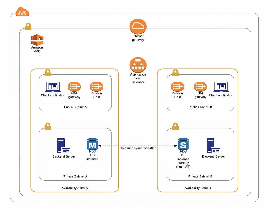
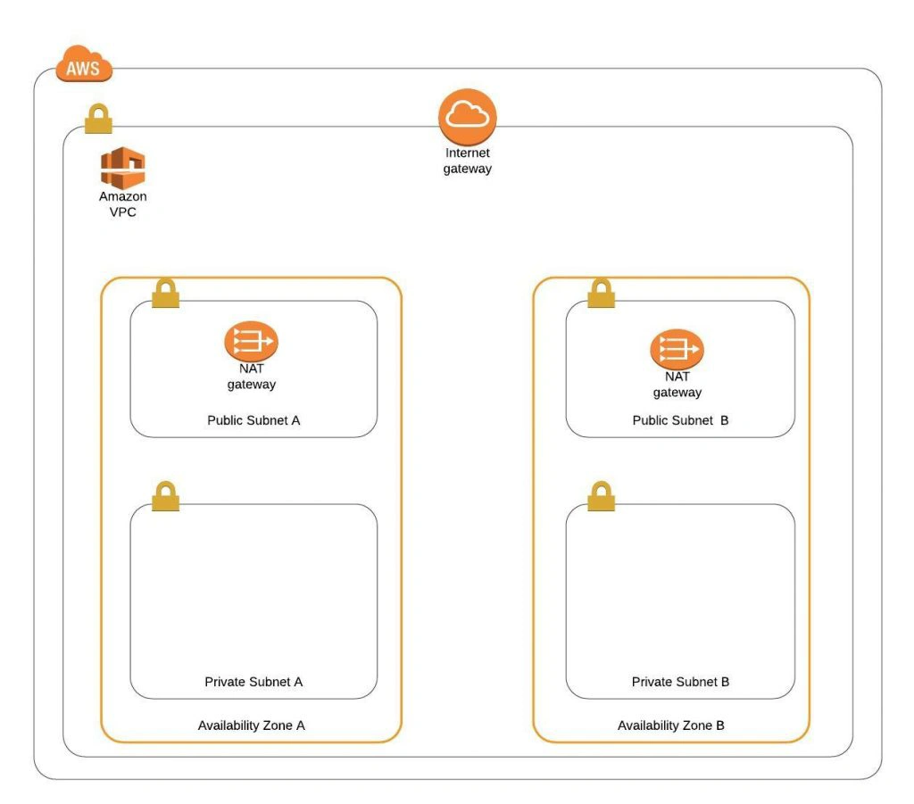
The architecture diagram is shown in figure 1. It comprises a VPC with four subnets (2 public and 2 private) distributed across two different availability zones. In public subnets are hosted a client application, a NAT gateway and a Bastion Host (more on that later), while our private subnets contain backend server and database instances. The infrastructure also includes Internet Gateway to enable access to the Internet from our VPC and a Load Balancer. The reasoning behind placing the backend server and database in private subnets is to protect those instances from being directly exposed to the Internet as they may contain sensitive data. Instead, they will only have private IP addresses and be behind a NAT gateway and a public-facing Elastic Load Balancer. Presented infrastructure provides a high level of scalability and availability through the introduction of redundancy with instances deployed in two different availability zones and the use of auto-scaling groups which provide automatic scaling and health management of the system.
Figure 2 presents the view of the user management web application system we will host on AWS:
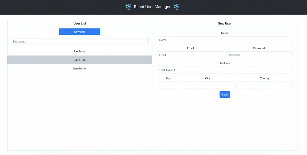
The applications can be found on GitHub.
In this part of the article series, we will focus on the scaffolding of the infrastructure, namely allocating elastic IP addresses, setting up the VPC, creating the subnets, configuring NAT gateways and route tables.
AWS Free Tier Note
AWS provides its new users with a 12-month free tier, which gives customers the ability to use their services up to specified limits free of charge. Those limits include 750 hours per month of t2.micro size EC2 instances, 5GB of Amazon S3 storage, 750 hours of Amazon RDS per month, and much more. In the AWS Management Console, Amazon usually provides indicators in which resource choices are part of the free tier, and throughout this series, we will stick to those. If you want to be sure you will not exceed the free tier limits, remember to stop your EC2 and RDS instances whenever you finish working on AWS. You can also set up a billing alert that will notify you if you exceed the specified limit.
AWS theory
1. VPC
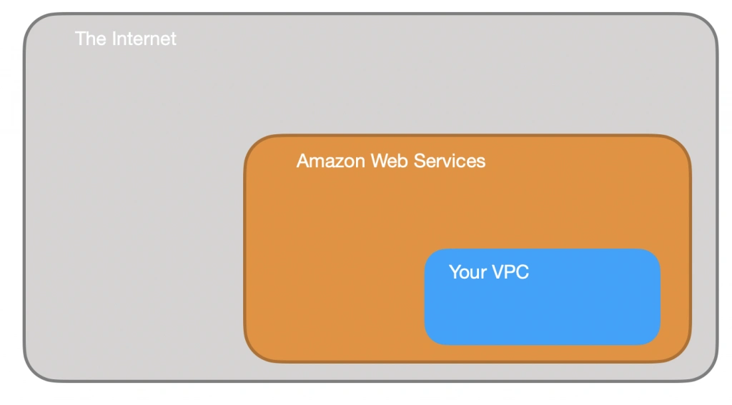
The first step of our journey into the wide world of the AWS infrastructure is getting to know Amazon Virtual Private Cloud (VPC). VPC allows developers to create a virtual network in which they can launch resources and have them logically isolated from other VPCs and the outside world. Within the VPC your resources have private IP addresses with which they can communicate with one another. You can control the access to all those resources inside the VPC and route outgoing traffic as you like.
Access to the VPC is configured with the use of several key structures:
Security groups - They basically work like mini firewalls defining allowed incoming and outgoing IP addresses and ports. They can be attached at the instance level, be shared among many instances and provide the possibility to allow access from other security groups instead of IPs.
Routing tables - Routing tables are responsible for determining where the network traffic from a subnet or gateway should be directed. There is a main route table associated with your VPC, and you can define custom routing tables for your subnets and gateways.
Network Access Control List (Network ACL) - It acts as an IP filtering table for incoming and outgoing traffic and can be used as an additional security layer on top of security groups. Network ACLs act similarly to the security groups, but instead of applying rules on the instance level, they apply them to the entire VPC or subnet.
2. Subnets
Instances cannot be launched directly into a VPC. They need to live inside subnets. A Subnet is an additional isolated area that has its own CIDR block, routing table, and Network Access Control List. Subnets allow you to create different behaviors in the same VPC. For instance, you can create a public subnet that can be accessed and have access to the public internet and a private subnet that is not accessible through the Internet and must go through a NAT (Network Address Translation) gateway in order to access the outside world.
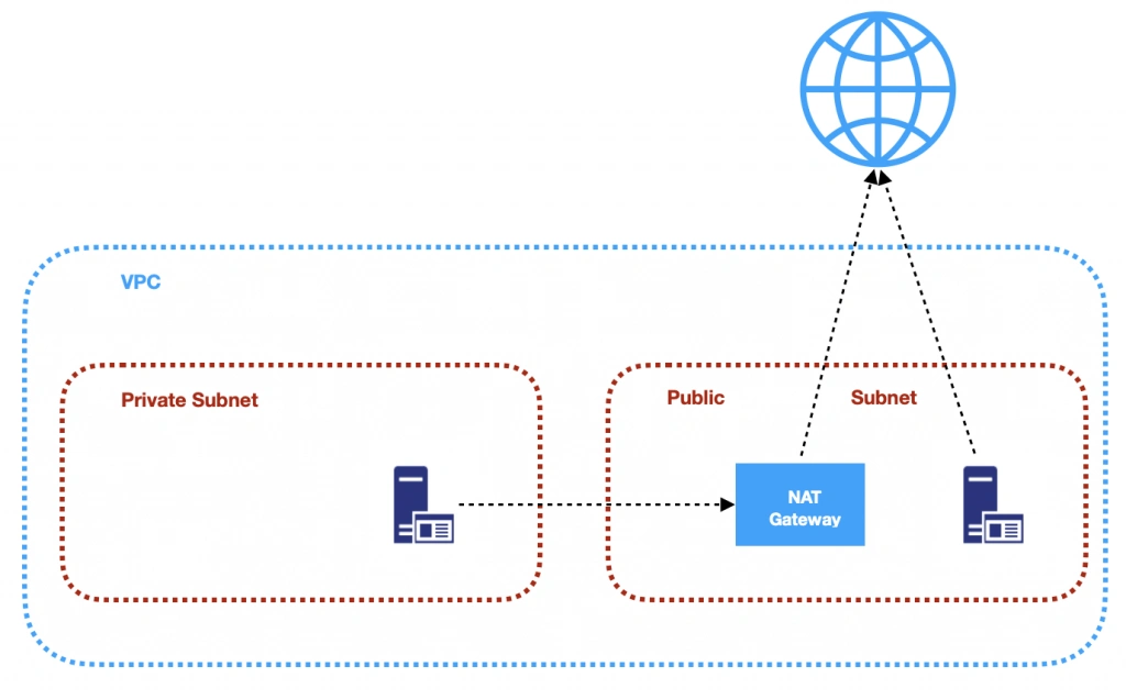
3. NAT (Network Address Transfer) gateway
NAT Gateways are used in order to enable instances located in private subnets to connect to the Internet or other AWS services, while still preventing direct connections from the Internet to those instances. NAT may be useful for example when you need to install or upgrade software or OS on EC2 instances running in private subnets. AWS provides a NAT gateway managed service which requires very little administrative effort. We will use it while setting up our infrastructure.
4. Elastic IP
AWS provides a concept of Elastic IP Address which is used to facilitate the management of dynamic cloud computing. Elastic IP Address is a public, static IP Address that is associated with your AWS account and can be easily allocated to one of your EC2 instances. The idea behind it is that the address is not strongly associated with your instance but instead elasticity of the address allows in a case of any failure in the system to swiftly remap the address to another healthy instance in your account.
5. AWS Region
AWS Regions are geographical areas in which AWS has data centers. Regions are divided into Availability Zones (AZ) which are independent data centers placed relatively close to each other. Availability Zones are used to provide redundancy and data replication. The choice of AWS region for your infrastructure should be determined to take into account factors such as:
- Proximity - you would usually want your application to be deployed close to your region of operation for latency or regulatory reasons.
- Cost - different regions come with different pricing.
- Feature selection - not all services are available in all regions, this is especially the case for newly introduced features.
- Several availability zones - all regions have at least 2 AZ, but some of them have more. Depending on your needs, this may be a key factor.
Practice
AWS Region
Let’s commence with a selection of the AWS region to operate in. In the top right corner of the AWS Management Console, you can choose a region. At this point, it does not really matter which region you choose (as discussed earlier, it may for your organization). However, it is important to note that you will always only view resources launched in the currently selected region.
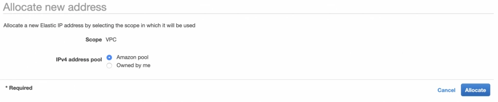
Elastic IP
The next step is the allocation of an elastic IP address. For that purpose, go into the AWS Management console, and find the VPC service. In the left menu bar, under the Virtual Private Cloud section, you should see the Elastic IPs link. There you can allocate a new address owned by yourself or from the pool of Amazon’s available addresses.
Availability Zone A configuration
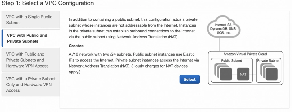
Next, let’s create our VPC and subnets. For now, we are going to set up only Availability Zone A and we will work on High Availability after the creation of the VPC. So go again into the VPC service dashboard and click the Launch VPC Wizard button. You will be taken to the screen where you can choose what kind of a VPC configuration you want Amazon to set you up with. In order to match our target architecture as closely as possible, we are going to choose VPC with Public and Private Subnets .
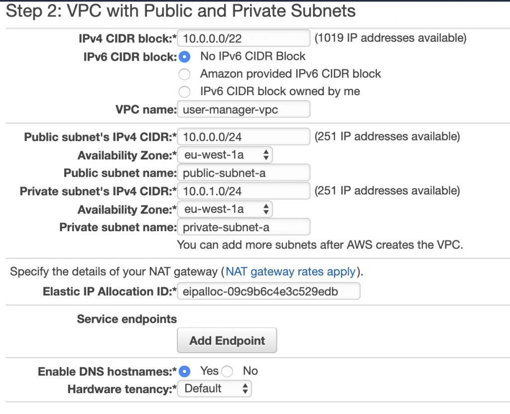
The next screen allows you to set up your VPC configuration details such as:
- name,
- CIDR block,
- details of the subnets:
- name,
- IP address range - a subset of the VPC CIDR range,
- availability zone,
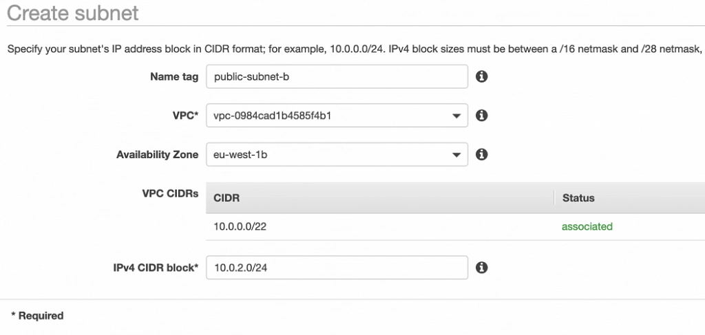
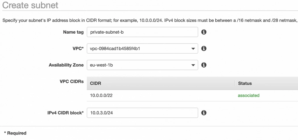
As shown in the architecture diagram (fig. 1), we need 4 subnets in 2 different availability zones. So let’s set our VPC CIDR to 10.0.0.0/22, and have our subnets as follows:
- public-subnet-a: 10.0.0.0/24 (zone A)
- private-subnet-a: 10.0.1.0/24 (zone A)
- public-subnet-b: 10.0.2.0/24 (zone B)
- private-subnet-b: 10.0.3.0/24 (zone B)
Set everything up as shown in figure 7. The important aspects to note here are the choice of the same availability zone for public and private subnets, and the fact that Amazon will automatically set us up with a NAT gateway for which we just need to specify our previously allocated Elastic IP Address. Now, click the Create VPC button, and Amazon will configure your VPC.
NAT gateway
When the creation of the VPC is over, go to the NAT Gateways section, and you should see the gateway created for you by AWS. To make it more recognizable, let us edit its Name tag to nat-a .

Route tables
Amazon also configured Route Tables for your VPC. Go to the Route Tables section, and you should have there two route tables associated with your VPC. One of them is the main route table of your VPC, and the second one is currently associated with your public-subnet-a. We will modify that setting a bit.
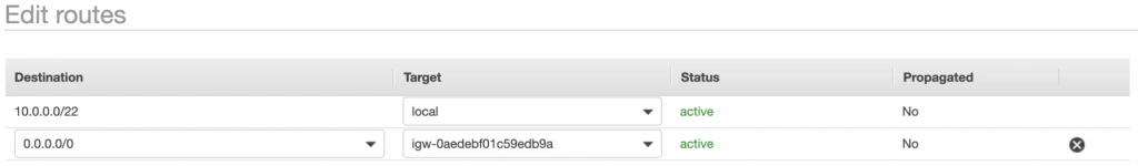
First, select the main route table, go to the routes tab and click Edit routes . There are currently two entries. The first one means Any IP address referencing local VPC CIDR should resolve locally and we shouldn’t modify it. The second one is pointing to the NAT gateway, but we will change it to configure the Internet Gateway of our VPC in order to let outgoing traffic reach the outside world.
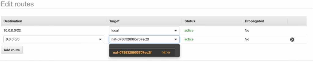
Next, go to the Subnet Associations tab and associate the main route table with public-subnet-a. You can also edit its Name tag to main-rt . Then, select the second route table associated with your VPC, edit its routes to route every outgoing Internet request to the nat-a gateway as shown in figure 10. Associate this route table with private-subnet-a and edit its Name tag to private-a-rt .
Availability Zone B Configuration
Well done, availability zone A is configured. In order to provide High Availability, we need to set everything up in the second availability zone as well. The first step is the creation of the subnets. Go again to a VPC dashboard in the AWS management console and in the left menu bar find the Subnets section. Now, click the Create subnet button and configure everything as shown in figures 11 and 12.
public-subnet-b
private-subnet-b
NAT gateway
For availability zone B we need to create the NAT gateway manually. For that, find the NAT Gateways section in the left menu bar of the VPC dashboard, and click Create NAT Gateway . Select public-subnet-b , allocate EIP and add a Name tag with value nat-b .
Route tables
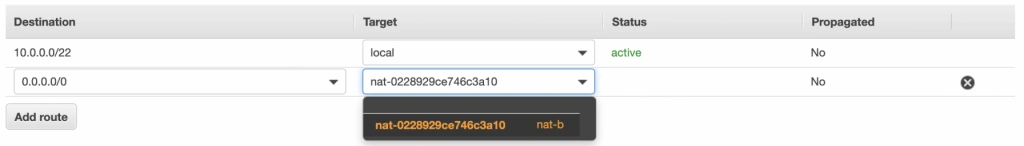
The last step is the configuration of the route tables for the subnets in availability zone B. For that, go to the Route Tables section again. Our public-subnet-b is going to have the same routing rules as the public-subnet-a, so let’s add a new association to our main-rt table for public-subnet-b. Then, click the Create route table button, name it private-b-rt , choose our VPC and click create . Next, select the newly created table go to the Routes tab and Edit routes by analogy with the private-a-rt table, but instead of directing every outside going request to nat-a gateway route it to nat-b (fig. 13).
In the end, you should have three route tables associated with your VPC as shown in figure 14.

Summary
That’s it, the scaffolding of our VPC is ready. The diagram shown in fig.15 presents a view of the created infrastructure. It is now ready for the creation of required EC2 instances, Bastion Hosts, configuration of an RDS database and deployment of our applications, which we will do in the next part of the series .
Sources:
- https://azure.microsoft.com/en-us/overview/what-is-cloud-computing/
- https://aws.amazon.com/what-is-aws/
- https://docs.aws.amazon.com/AWSEC2/latest/UserGuide/elastic-ip-addresses-eip.html
- https://docs.aws.amazon.com/vpc/latest/userguide/VPC_Route_Tables.html
- https://docs.aws.amazon.com/vpc/latest/userguide/VPC_SecurityGroups.html#DefaultSecurityGroup
- https://docs.aws.amazon.com/vpc/latest/userguide/vpc-network-acls.html
- https://medium.com/@datapath_io/elastic-ip-static-ip-public-ip-whats-the-difference-8e36ac92b8e7
- https://cloudacademy.com/blog/aws-bastion-host-nat-instances-vpc-peering-security/
- https://aws.amazon.com/blogs/aws/internal-elastic-load-balancers/
- https://aws.amazon.com/quickstart/architecture/linux-bastion/
- https://aws.amazon.com/blogs/security/securely-connect-to-linux-instances-running-in-a-private-amazon-vpc/
- http://thebluenode.com/exposing-private-ec2-instances-behind-public-elastic-load-balancer-elb-aws
- https://app.pluralsight.com/library/courses/aws-developer-getting-started/table-of-contents
- https://app.pluralsight.com/library/courses/aws-developer-designing-developing/table-of-contents
- https://app.pluralsight.com/library/courses/aws-networking-deep-dive-vpc/table-of-contents
- https://datanextsolutions.com/blog/using-nat-gateways-in-aws/
- https://docs.aws.amazon.com/vpc/latest/userguide/vpc-nat-gateway.html
Interested in our services?
Reach out for tailored solutions and expert guidance.