How to automate operationalization of Machine Learning apps - an introduction to Metaflow

In this article, we briefly highlight the features of Metaflow, a tool designed to help data scientists operationalize machine learning applications.
Introduction to machine learning operationalization
Data-driven projects become the main area of focus for a fast-growing number of companies. The magic has started to happen a couple of years ago thanks to sophisticated machine learning algorithms, especially those based on deep learning. Nowadays, most companies want to use that magic to create software with a breeze of intelligence. In short, there are two kinds of skills required to become a data wizard:
Research skills - understood as the ability to find typical and non-obvious solutions for data-related tasks, specifically extraction of knowledge from data in the context of a business domain. This job is typically done by data scientists but is strongly related to machine learning, data mining, and big data.
Software engineering skills - because the matter in which these wonderful things can exist is software. No matter what we do, there are some rules of the modern software development process that help a lot to be successful in business. By analogy with intelligent mind and body, software also requires hardware infrastructure to function.
People tend to specialize, so over time, a natural division has emerged between those responsible for data analysis and those responsible for transforming prototypes into functional and scalable products. That shouldn't be surprising, as creating rules for a set of machines in the cloud is a far different job from the work of a data detective.
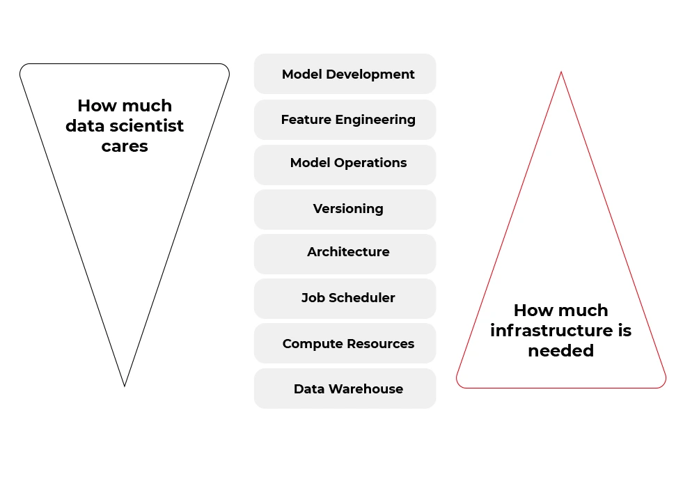
Fortunately, many of the tasks from the second bucket (infrastructure and software) can be automated. Some tools aim to boost the productivity of data scientists by allowing them to focus on the work of a data detective rather than on the productionization of solutions. And one of these tools is called Metaflow.
If you want to focus more on data science , less on engineering, but be able to scale every aspect of your work with no pain, you should take a look at how is Metaflow designed.
A Review of Metaflow
Metaflow is a framework for building and managing data science projects developed by Netflix. Before it was released as an open-source project in December 2019, they used it to boost the productivity of their data science teams working on a wide variety of projects from classical statistics to state-of-the-art deep learning.

The Metaflow library has Python and R API, however, almost 85% of the source code from the official repository (https://github.com/Netflix/metaflow) is written in Python. Also, separate documentation for R and Python is available.
At the time this article is written (July 2021), the official repository of the Metaflow has 4,5 k stars, above 380 forks, and 36 contributors, so it can be assumed as a mature framework.
“Metaflow is built for data scientists, not just for machines”
That sentence got attention when you visit the official website of the project ( https://metaflow.org/ ). Indeed, these are not empty words. Metaflow takes care of versioning, dependency management, computing resources, hyperparameters, parallelization, communication with AWS stack, and much more. You can truly focus on the core part of your data-related work and let Metaflow do all these things using just very expressive decorators.
Metaflow - core features
The list below explains the key features that make Metaflow such a wonderful tool for data scientists, especially for those who wish to remain ignorant in other areas.
- Abstraction over infrastructure. Metaflow provides a layer of abstraction over the hardware infrastructure available, cloud stack in particular. That’s why this tool is sometimes called a unified API to the infrastructure stack.
- Data pipeline organization. The framework represents the data flow as a directed acyclic graph. Each node in the graph, also called step, contains some code to run wrapped in a function with @step decorator.
@step
def get_lat_long_features(self):
self.features = coord_features(self.data, self.features)
self.next(self.add_categorical_features)
The nodes on each level of the graph can be computed in parallel, but the state of the graph between levels must be synchronized and stored somewhere (cached) – so we have very good asynchronous data pipeline architecture.

This approach facilitates debugging, enhances the performance of the pipeline, and allows us completely separate the steps so that we can run one step locally and the next one in the cloud if, for instance, the step requires solving large matrices. The disadvantage of that approach is that salient failures may happen without proper programming discipline.
- Versioning. Tracking versions of our machine learning models can be a challenging task. Metaflow can help here. The execution of each step of the graph (data, code, and parameters) is hashed and stored, and you can access logged data later, using client API.
- Containerization. Each step is run in a separate environment. We can specify conda libraries in each container using
@condadecorator as shown below. It can be a very useful feature under some circumstances.
@conda(libraries={"scikit-learn": "0.19.2"})
@step
def fit(self):
...
- Scalability. With the help of
@batchand@resourcesdecorators, we can simply command AWS Batch to spawn a container on ECS for the selected Metaflow step. If individual steps take long enough, the overhead of spawning the containers should become irrelevant.
@batch(cpu=1, memory=500)
@step
def hello(self):
...
- Hybrid runs. We can run one step locally and another compute-intensive step on the cloud and swap between these two modes very easily.
- Error handling. Metaflow’s
@retrydecorator can be used to set the number of retries if the step fails. Any error raised during execution can be handled by@catchdecorator. The@timeoutdecorator can be used to limit long-running jobs especially in expensive environments (for example with GPGPUs).
@catch(var="compute_failed")
@retry
@step
def statistics(self):
...
- Namespaces. An isolated production namespace helps to keep production results separate from experimental runs of the same project running concurrently. This feature is very useful in bigger projects where more people is involved in development and deployment processes.
from metaflow import Flow, namespace
namespace("user:will")
run = Flow("PredictionFlow").latest_run
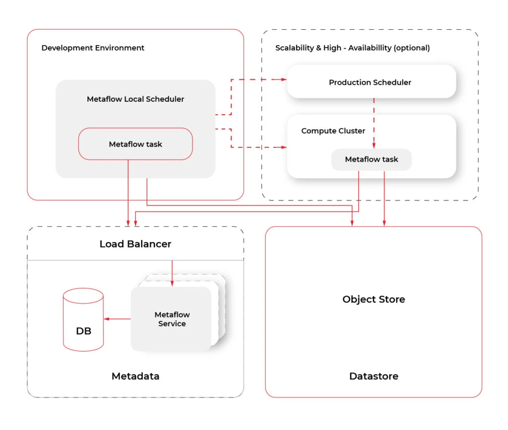
- Cloud Computing . Metaflow, by default, works in the local mode . However, the shared mode releases the true power of Metaflow. At the moment of writing, Metaflow is tightly and well coupled to AWS services like CloudFormation, EC2, S3, Batch, DynamoDB, Sagemaker, VPC Networking, Lamba, CloudWatch, Step Functions and more. There are plans to add more cloud providers in the future. The diagram below shows an overview of services used by Metaflow.
Metaflow - missing features
Metaflow does not solve all problems of data science projects. It’s a pity that there is only one cloud provider available, but maybe it will change in the future. Model serving in production could be also a really useful feature. Competitive tools like MLFlow or Apache AirFlow are more popular and better documented. Metaflow lacks a UI that would make metadata, logging, and tracking more accessible to developers. All this does not change the fact that Metaflow offers a unique and right approach, so just cannot be overlooked.
Conclusions
If you think Metaflow is just another tool for MLOps , you may be surprised. Metaflow offers data scientists a very comfortable workflow abstracting them from all low levels of that stuff. However, don't expect the current version of Metaflow to be perfect because Metaflow is young and still actively developed. However, the foundations are solid, and it has proven to be very successful at Netflix and outside of it many times.

Grape Up guides enterprises on their data-driven transformation journey
Ready to ship? Let's talk.
Check related articles
Read our blog and stay informed about the industry's latest trends and solutions.
Train your computer with the Julia programming language - introduction
As the Julia programming language is becoming very popular in building machine learning applications, we explain its advantages and suggest how to leverage them.
Python and its ecosystem have dominated the machine learning world – that’s an undeniable fact. And it happened for a reason. Ease of use and simple syntax undoubtedly contributed to still growing popularity. The code is understandable by humans, and developers can focus on solving an ML problem instead of focusing on the technical nuances of the language. But certainly, the most significant source of technology success comes from community effort and the availability of useful libraries.
In that context, the Python environment really shines. We can google in five seconds a possible solution for a great majority of issues related to the language, libraries, and useful examples, including theoretical and practical aspects of our intelligent application or scientific work. Most of the machine learning related tutorials and online courses are embedded in the Python ecosystem. If some ML or AI algorithm is worth of community’s attention, there is a huge probability that somebody implemented it as a Python open-source library.
Python is also the "Programming Language of the 2020" award winner. The award is given to the programming language that has the highest rise in ratings in a year based on the TIOBE programming community index (a measure of the popularity of programming languages). It is worth noting that the rise of Python language popularity is strongly correlated with the rise of machine learning popularity.
Equipped with such great technology, why still are we eager to waste a lot of our time looking for something better? Except for such reasons as being bored or the fact that many people don’t like snakes (although the name comes from „Monty Python’s Flying Circus”, a python still remains a snake). We think that the answer is quite simple: because we can do it better.
From Python to Julia
To understand that there is a potential to improve, we can go back to the early nineties when Python was created. It was before 3rd wave of artificial intelligence popularity and before the exponential increase in interest in deep learning. Some hard-to-change design decisions that don’t fit modern machine learning approaches were unavoidable. Python is old, it’s a fact, a great advantage, but also a disadvantage. A lot of great and groundbreaking things happened from the times when Python was born.
While Python has dominated the ML world, a great alternative has emerged for anyone who expects more. The Julia Language was created in 2009 by a four-person team from MIT and released in 2012. The authors wanted to address the shortcomings in Python and other languages. Also, as they were scientists, they focused on scientific and numerical computation, hitting a niche occupied by MATLAB, which is very good for that application but is not free and not open source. The Julia programming language combines the speed of C with the ease of use of Python to satisfy both scientists and software developers. And it integrates with all of them seamlessly.
In the following sections, we will show you how the Julia Language can be adapted to every Machine Learning problem . We will cover the core features of the language shown in the context of their usefulness in machine learning and comparison with other languages. A short overview of machine learning tools and frameworks available in Julia is also included. Tools for data preparation, visualization of results, and creating production pipelines also are covered. You will see how easily you can use ML libraries written in other languages like Python, MATLAB, or C/C++ using powerful metaprogramming features of the Julia language. The last part presents how to use Julia in practice, both for rapid prototyping and building cloud-based production pipelines.
The Julia language
Someone said if Python is a premium BMW sedan (petrol only, I guess, eventual hybrid) then Julia is a flagship Tesla. BMW has everything you need, but more and more people are buying Tesla. I can somehow agree with that, and let me explain the core features of the language which makes Julia so special and let her compete for a place in the TIOBE ranking with such great players as LISP, Scala, or Kotlin (31st place in March 2021).
Unusual JIT/AOT complier
Julia uses the LLVM compiler framework behind the scenes to translate very simple and dynamic syntax into machine code. This happens in two main steps. The first step is precompilation, before final code execution, and what may be surprising this it actually runs the code and stores some precompilation effects in the cache. It makes runtime faster but slower building – usually this is an acceptable cost.
The second step occurs in runtime. The compiler generates code just before execution based on runtime types and static code analysis. This is not how traditional just-in-time compilers work e.g., in Java. In “pure” JIT the compiler is not invoked until after a significant number of executions of the code to be compiled. In that context, we can say that Julia works in much the same way as C or C++. That’s why some people call Julia compiler a just-ahead-of-time compiler, and that’s why Julia can run near as fast as C in many cases while remaining a dynamic language like Python. And this is just awesome.
Read-eval-print loop
Read-eval-print loop (REPL) is an interactive command line that can be found in many modern programming languages. But in the case of Julia, the REPL can be used as the real heart of the entire development process. It lets you manage virtual environments, offers a special syntax for the package manager, documentation, and system shell interactions, allows you to test any part of your code, the language, libraries, and many more.
Friendly syntax
The syntax is similar to MATLAB and Python but also takes the best of other languages like LISP. Scientists will appreciate that Unicode characters can be used directly in source code, for example, this equation: f(X,u,σᵀ∇u,p,t) = -λ * sum(σᵀ∇u.^2)
is a perfectly valid Julia code. You may notice how cool it can be in terms of machine learning. We use these symbols in machine learning related books and articles, why not use them in source code?
Optional typing
We can think of Julia as dynamically typed but using type annotation syntax, we can treat variables as being statically typed, and improve performance in cases where the compiler could not automatically infer the type. This approach is called optional typing and can be found in many programming languages. In Julia however, if used properly, can result in a great boost of performance as this approach fits very well with the way Julia compiler works.
A ‘Glue’ language
Julia can interface directly with external libraries written in C, C++, and Fortran without glue code. Interface with Python code using PyCall library works so well that you can seamlessly use almost all the benefits of great machine learning Python ecosystem in Julia project as if it were native code! For example, you can write:
np = pyimport(numpy)
and use numpy in the same way you do with Python using Julia syntax. And you can configure a separate miniconda Python interpreter for each project and set up everything with one command as with Docker or similar tools. There are bindings to other languages as well e.g., Java, MATLAB, or R.
Julia supports metaprogramming
One of Julia's biggest advantages is Lisp-inspired metaprogramming. A very powerful characteristic called homoiconicity explained by a famous sentence: “code is data and data is code” allows Julia programs to generate other Julia programs, and even modify their own code. This approach to metaprogramming gives us so much flexibility, and that’s how developers do magic in Julia.
Functional style
Julia is not an object-oriented language. Something like a model.fit() function call is possible (Julia is very flexible) but not common in Julia. Instead, we write fit(model) , and it's not about the syntax, but it is about the organization of all code in our program (modules, multiple dispatches, functions as a first-class citizen, and many more).
Parallelization and distributed computing
Designed with ML in mind, Julia focusses on the scientific computing domain and its needs like parallel, distributed intensive computation tasks. And the syntax is very easy for local or remote parallelism.
Disadvantages
Well, it might be good if the compiler wasn't that slow, but it keeps getting better. Sometimes REPL could be faster, but again it’s getting better, and it depends on the host operating system.
Conclusion
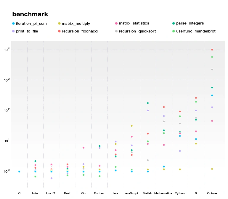
By concluding this section, we would like to demonstrate a benchmark comparing several popular languages and Julia. All language benchmarks should be treated not too seriously, but they still give an approximate view of the situation.
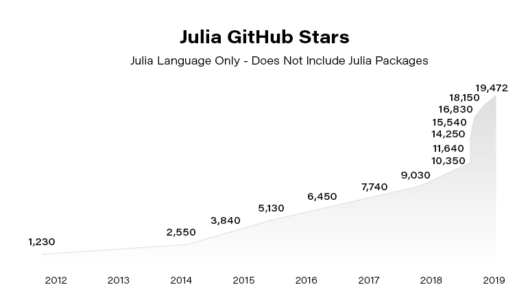
Julia becomes more and more popular. Since the 2012 launch, Julia has been downloaded over 25,000,000 times as of February 2021, up by 87% in a year.
In the next article, we focus on using Julia in building Machine Learning models. You can also check our guide to getting started with the language .
Getting started with the Julia language
Are you looking for a programming language that is fast, easy to start with, and trending? The Julia language meets the requirements. In this article, we show you how to take your first steps.
What is the Julia language?
Julia is an open-source programming language for general purposes. However, it is mainly used for data science, machine learning , or numerical and statistical computing. It is gaining more and more popularity. According to the TIOBE index, the Julia language jumped from position 47 to position 23 in 2020 and is highly expected to head towards the top 20 next year.
Despite the fact Julia is a flexible dynamic language, it is extremely fast. Well-written code is usually as fast as C, even though it is not a low-level language. It means it is much faster than languages like Python or R, which are used for similar purposes. High performance is achieved by using type interference and JIT (just-in-time) compilation with some AOT (ahead-of-time) optimizations. You can directly call functions from other languages such as C, C++, MATLAB, Python, R, FORTRAN… On the other hand, it provides poor support for static compilation, since it is compiled at runtime.
Julia makes it easy to express many object-oriented and functional programming patterns. It uses multiple dispatches, which is helpful, especially when writing a mathematical code. It feels like a scripting language and has good support for interactive use. All those attributes make Julia very easy to get started with and experiment with.
First steps with the Julina language
- Download and install Julia from Download Julia .
- (Optional - not required to follow the article) Choose your IDE for the Julia language. VS Code is probably the most advanced option available at the moment of writing this paragraph. We encourage you to do your research and choose one according to your preferences. To install VSCode, please follow Installing VS Code and VS Code Julia extension .
Playground
Let’s start with some experimenting in an interactive session. Just run the Julia command in a terminal. You might need to add Julia's binary path to your PATH variable first. This is the fastest way to learn and play around with Julia.
C:\Users\prso\Desktop>julia
_
_ _ _(_)_ | Documentation: https://docs.julialang.org
(_) | (_) (_) |
_ _ _| |_ __ _ | Type "?" for help, "]?" for Pkg help.
| | | | | | |/ _` | |
| | |_| | | | (_| | | Version 1.5.3 (2020-11-09)
_/ |\__'_|_|_|\__'_| | Official https://julialang.org/ release
|__/ |
julia> println("hello world")
hello world
julia> 2^10
1024
julia> ans*2
2048
julia> exit()
C:\Users\prso\Desktop>
To get a recently returned value, we can use the ans variable. To close REPL, use exit() function or Ctrl+D shortcut.
Running the scripts
You can create and run your scripts within an IDE. But, of course, there are more ways to do so. Let’s create our first script in any text editor and name it: example.jl.
x = 2
println(10x)
You can run it from REPL:
julia> include("example.jl")
20
Or, directly from your system terminal:
C:\Users\prso\Desktop>julia example.jl
20
Please be aware that REPL preserves the current state and includes statement works like a copy-paste. It means that running included is the equivalent of typing this code directly in REPL. It may affect your subsequent commands.
Basic types
Julia provides a broad range of primitive types along with standard mathematical functions and operators. Here’s the list of all primitive numeric types:
- Int8, UInt8
- Int16, UInt16
- Int32, UInt32
- Int64, UInt64
- Int128, UInt128
- Float16
- Float32
- Float64
A digit suffix implies several bits and a U prefix that is unsigned. It means that UInt64 is unsigned and has 64 bits. Besides, it provides full support for complex and rational numbers.
It comes with Bool , Char , and String types along with non-standard string literals such as Regex as well. There is support for non-ASCII characters. Both variable names and values can contain such characters. It can make mathematical expressions very intuitive.
julia> x = 'a'
'a': ASCII/Unicode U+0061 (category Ll: Letter, lowercase)
julia> typeof(ans)
Char
julia> x = 'β'
'β': Unicode U+03B2 (category Ll: Letter, lowercase)
julia> typeof(ans)
Char
julia> x = "tgα * ctgα = 1"
"tgα * ctgα = 1"
julia> typeof(ans)
String
julia> x = r"^[a-zA-z]{8}$"
r"^[a-zA-z]{8}$"
julia> typeof(ans)
Regex
Storage: Arrays, Tuples, and Dictionaries
The most commonly used storage types in the Julia language are: arrays, tuples, dictionaries, or sets. Let’s take a look at each of them.
Arrays
An array is an ordered collection of related elements. A one-dimensional array is used as a vector or list. A two-dimensional array acts as a matrix or table. More dimensional arrays express multi-dimensional matrices.
Let’s create a simple non-empty array:
julia> a = [1, 2, 3]
3-element Array{Int64,1}:
1
2
3
julia> a = ["1", 2, 3.0]
3-element Array{Any,1}:
"1"
2
3.0
Above, we can see that arrays in Julia might store Any objects. However, this is considered an anti-pattern. We should store specific types in arrays for reasons of performance.
Another way to make an array is to use a Range object or comprehensions (a simple way of generating and collecting items by evaluating an expression).
julia> typeof(1:10)
UnitRange{Int64}
julia> collect(1:3)
3-element Array{Int64,1}:
1
2
3
julia> [x for x in 1:10 if x % 2 == 0]
5-element Array{Int64,1}:
2
4
6
8
10
We’ll stop here. However, there are many more ways of creating both one and multi-dimensional arrays in Julia.
There are a lot of built-in functions that operate on arrays. Julia uses a functional style unlike dot-notation in Python. Let’s see how to add or remove elements.
julia> a = [1,2]
2-element Array{Int64,1}:
1
2
julia> push!(a, 3)
3-element Array{Int64,1}:
1
2
3
julia> pushfirst!(a, 0)
4-element Array{Int64,1}:
0
1
2
3
julia> pop!(a)
3
julia> a
3-element Array{Int64,1}:
0
1
2
Tuples
Tuples work the same way as arrays. A tuple is an ordered sequence of elements. However, there is one important difference. Tuples are immutable. Trying to call methods like push!() will result in an error.
julia> t = (1,2,3)
(1, 2, 3)
julia> t[1]
1
Dictionaries
The next commonly used collections in Julia are dictionaries. A dictionary is called Dict for short. It is, as you probably expect, a key-value pair collection.
Here is how to create a simple dictionary:
julia> d = Dict(1 => "a", 2 => "b")
Dict{Int64,String} with 2 entries:
2 => "b"
1 => "a"
julia> d = Dict(x => 2^x for x = 0:5)
Dict{Int64,Int64} with 6 entries:
0 => 1
4 => 16
2 => 4
3 => 8
5 => 32
1 => 2
julia> sort(d)
OrderedCollections.OrderedDict{Int64,Int64} with 6 entries:
0 => 1
1 => 2
2 => 4
3 => 8
4 => 16
5 => 32
We can see, that dictionaries are not sorted. They don’t preserve any particular order. If you need that feature, you can use SortedDict .
julia> import DataStructures
julia> d = DataStructures.SortedDict(x => 2^x for x = 0:5)
DataStructures.SortedDict{Any,Any,Base.Order.ForwardOrdering} with 6 entries:
0 => 1
1 => 2
2 => 4
3 => 8
4 => 16
5 => 32
DataStructures is not an out-of-the-box package. To use it for the first time, we need to download it. We can do it with a Pkg package manager.
julia> import Pkg; Pkg.add("DataStructures")
Sets
Sets are another type of collection in Julia. Just like in many other languages, Set doesn’t preserve the order of elements and doesn’t store duplicated items. The following example creates a Set with a specified type and checks if it contains a given element.
julia> s = Set{String}(["one", "two", "three"])
Set{String} with 3 elements:
"two"
"one"
"three"
julia> in("two", s)
true
This time we specified a type of collection explicitly. You can do the same for all the other collections as well.
Functions
Let’s recall what we learned about quadratic equations at school. Below is an example script that calculates the roots of a given equation: ax2+bx+c .
discriminant(a, b, c) = b^2 - 4a*c
function rootsOfQuadraticEquation(a, b, c)
Δ = discriminant(a, b, c)
if Δ > 0
x1 = (-b - √Δ)/2a
x2 = (-b + √Δ)/2a
return x1, x2
elseif Δ == 0
return -b/2a
else
x1 = (-b - √complex(Δ))/2a
x2 = (-b + √complex(Δ))/2a
return x1, x2
end
end
println("Two roots: ", rootsOfQuadraticEquation(1, -2, -8))
println("One root: ", rootsOfQuadraticEquation(2, -4, 2))
println("No real roots: ", rootsOfQuadraticEquation(1, -4, 5))
There are two functions. The first one is just a one-liner and calculates a discriminant of the equation. The second one computes the roots of the function. It returns either one value or multiple values using tuples.
We don’t need to specify argument types. The compiler checks those types dynamically. Please take note that the same happens when we call sqrt() function using a √ symbol. In that case, when the discriminant is negative, we need to wrap it with a complex()function to be sure that the sqrt() function was called with a complex argument.
Here is the console output of the above script:
C:\Users\prso\Documents\Julia>julia quadraticEquations.jl
Two roots: (-2.0, 4.0)
One root: 1.0
No real roots: (2.0 - 1.0im, 2.0 + 1.0im)
Plotting
Plotting with the Julia language is straightforward. There are several packages for plotting. We use one of them, Plots.jl.
To use it for the first, we need to install it:
julia> using Pkg; Pkg.add("Plots")
After the package was downloaded, let’s jump straight to the example:
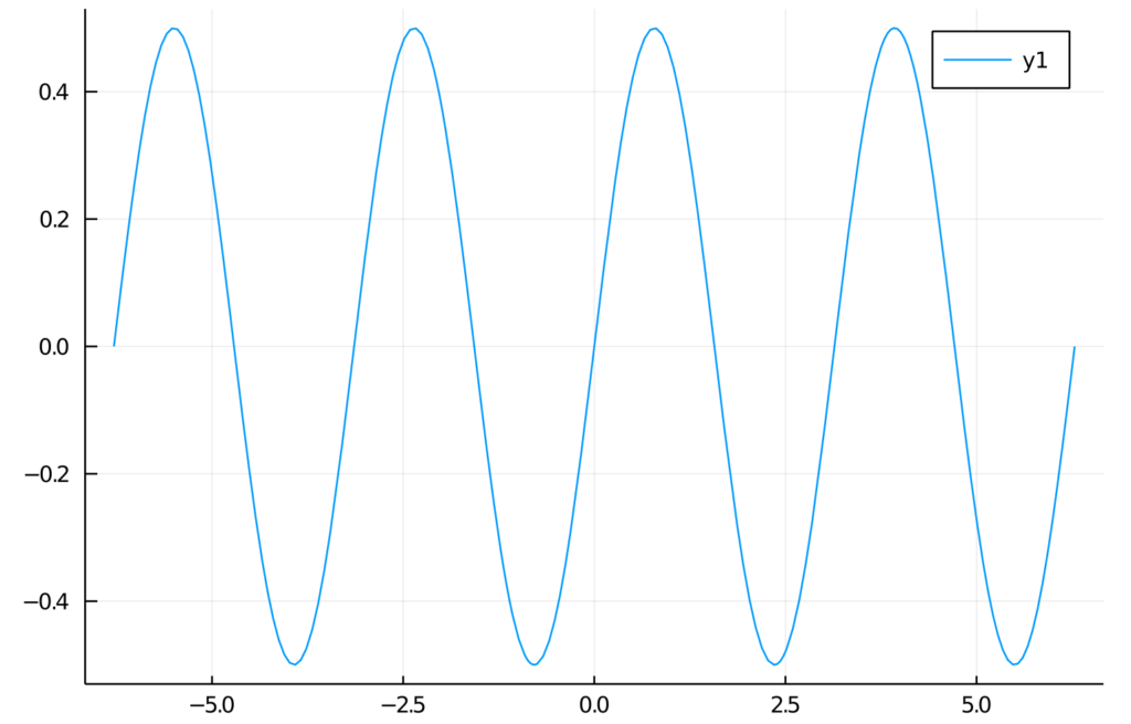
julia> f(x) = sin(x)cos(x)
f (generic function with 1 method)
julia> plot(f, -2pi, 2pi)
We’re expecting a graph of a function in a range from -2π to 2π. Here is the output:
Summary and further reading
In this article, we learned how to get started with Julia. We installed all the required components. Then we wrote our first “hello world” and got acquainted with basic Julia elements.
Of course, there is no way to learn a new language from reading one article. Therefore, we encourage you to play around with the Julia language on your own.
To dive deeper, we recommend reading the following sources:
How to automate operationalization of Machine Learning apps - running first project using Metaflow
In the second article of the series, we guide you on how to run a simple project in an AWS environment using Metaflow. So, let’s get started.
Need an introduction to Metaflow? Here is our article covering basic facts and features .
Prerequisites
- Python 3
- Miniconda
- Active AWS subscription
Installation
To install Metaflow, just run in the terminal:
conda config --add channels conda-forge conda install -c conda-forge metaflow
and that's basically it. Alternatively, if you want to only use Python without conda type:
pip install metaflow
Set the following environmental variables related to your AWS account:
- AWS_ACCESS_KEY_ID
- AWS_SECRET_ACCESS_KEY
- AWS_DEFAULT_REGION
AWS Server-Side configuration
The separate documentation called “ Administrator's Guide to Metaflow “ explains in detail how to configure all the AWS resources needed to enable cloud scaling in Metaflow. The easier way is to use the CloudFormation template that deploys all the necessary infrastructure. The template can be found here . If for some reason, you can’t or don’t want to use the CloudFormation template, the documentation also provides detailed instructions on how to deploy necessary resources manually. It can be a difficult task for anyone who’s not familiar with AWS services so ask your administrator for help if you can. If not, then using the CloudFormation template is a much better option and in practice is not so scary.
AWS Client-Side configuration
The framework needs to be informed about the surrounding AWS services. Doing it is quite simple just run:
metaflow configure aws
in terminal. You will be prompted for various resource parameters like S3, Batch Job Queue, etc. This command explains in short what’s going on, which is really nice. All parameters will be stored under the ~/.metaflowconfig directory as a json file so you can modify it manually also. If you don’t know what should be the correct input for prompted variables, in the AWS console, go to CloudFormation -> Stacks -> YourStackName -> Output and check all required values there. The output of the stack formation will be available after the creation of your stack from the template as explained above. After that, we are ready to use Metaflow in the cloud!
Hello Metaflow
Let's write very simple Python code to see what boilerplate we need to create a minimal working example.
hello_metaflow.py
from metaflow import FlowSpec, step
class SimpleFlow(FlowSpec):
@step
def start(self):
print('Lets start the flow!')
self.message = 'start message'
print(self.message)
self.next(self.modify_message)
@step
def modify_message(self):
self.message = 'modified message'
print(self.message)
self.next(self.end)
@step
def end(self):
print('The class members are shared between all steps.')
print(self.message)
if __name__ == '__main__':
SimpleFlow()
The designers of Metaflow decided to apply an object-oriented approach. To create a flow, we must create a custom class that inherits from FlowSpec class. Each step in our pipeline is marked by @step decorator and basically is represented by a member function. Use self.next member function to specify the flow direction in the graph. As we mentioned before, this is a directed acyclic graph – no cycles are allowed, and the flow must go in one way, with no backward movement. Steps named start and end are required to define the endpoints of the graph. This code results in a graph with three nodes and two-edged.

It’s worth to note that when you assign anything to self in your flow, the object gets automatically persisted in S3 as a Metaflow artifact.
To run our hello world example, just type in the terminal:
python3 hello_metaflow.py run
Execution of the command above results in the following output:
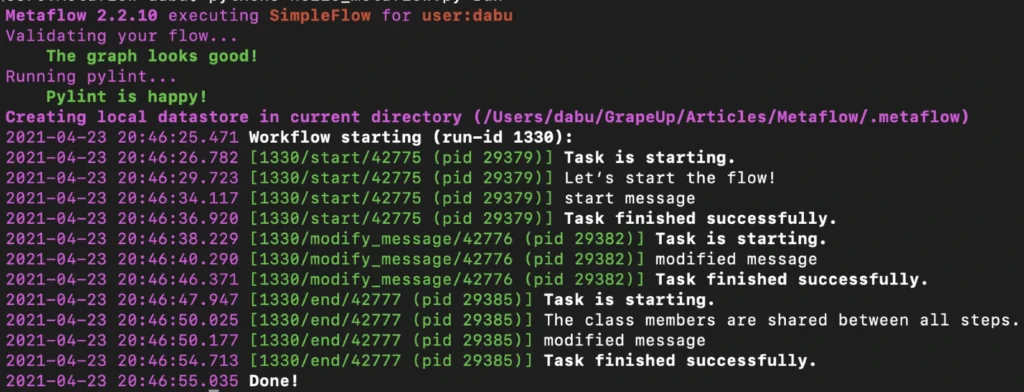
By default, Metaflow uses local mode . You may notice that in this mode, each step spawns a separate process with its own PID. Without much effort, we have obtained code that can be very easily paralleled on your personal computer.
To print the graph in the terminal, type the command below.
python3 hello_metaflow.py show
Let’s modify hello_metaflow.py script so that it imitates the training of the model.
hello_metaflow.py
from metaflow import FlowSpec, step, batch, catch, timeout, retry, namespace
from random import random
class SimpleFlow(FlowSpec):
@step
def start(self):
print('Let’s start the parallel training!')
self.parameters = [
'first set of parameters',
'second set of parameters',
'third set of parameters'
]
self.next(self.train, foreach='parameters')
@catch(var = 'error')
@timeout(seconds = 120)
@batch(cpu = 3, memory = 500)
@retry(times = 1)
@step
def train(self):
print(f'trained with {self.input}')
self.accuracy = random()
self.set_name = self.input
self.next(self.join)
@step
def join(self, inputs):
top_accuracy = 0
for input in inputs:
print(f'{input.set_name} accuracy: {input.accuracy}')
if input.accuracy > top_accuracy:
top_accuracy = input.accuracy
self.winner = input.set_name
self.winner_accuracy = input.accuracy
self.next(self.end)
@step
def end(self):
print(f'The winner is: {self.winner}, acc: {self.winner_accuracy}')
if __name__ == '__main__':
namespace('grapeup')
SimpleFlow()
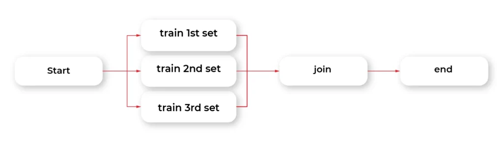
The start step prepares three sets of parameters for our dummy training. The optional argument for each passed to the next function call splits our graph into three parallel nodes. Foreach executes parallel copies of the train step.
The train step is the essential part of this example. The @batch decorator sends out parallel computations to the AWS nodes in the cloud using the AWS Batch service. We can specify how many virtual CPU cores we need, or the amount of RAM required. This one line of Python code allows us to run heavy computations in parallel nodes in the cloud at a very large scale without much effort. Simple, isn't it?
The @catch decorator catches the exception and stores it in an error variable, and lets the execution continue. Errors can be handled in the next step. You can also enable retries for a step simply by adding @retry decorator. By default, there is no timeout for steps, so it potentially can cause an infinite loop. Metaflow provides a @timeout decorator to break computations if the time limit is exceeded.
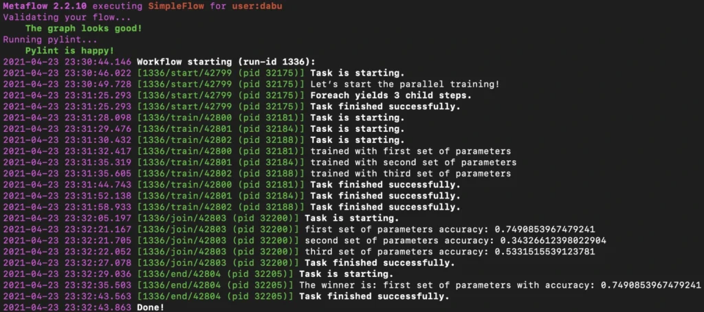
When all parallel pieces of training in the cloud are complete, we merge the results in the join function. The best solution is selected and printed as the winner in the last step.
Namespaces is a really useful feature that helps keeping isolated different runs environments, for instance, production and development environments.
Below is the simplified output of our hybrid training.
Obviously, there is an associated cost of sending computations to the cloud, but usually, it is not significant, and the benefits of such a solution are unquestionable.
Metaflow - Conclusions
In the second part of the article about Metaflow, we presented only a small part of the library's capabilities. We encourage you to read the documentation and other studies. We will only mention here some interesting and useful functionalities like passing parameters, conda virtual environments for a given step, client API, S3 data management, inspecting flow results with client API, debugging, workers and runs management, scheduling, notebooks, and many more. We hope this article has sparked your interest in Metaflow and will encourage you to explore this area further.
Interested in our services?
Reach out for tailored solutions and expert guidance.