Thinking out loud

This article is the second one of the mini-series which will help you to get familiar with RSocket – a new binary protocol which may revolutionize machine to machine communication in distributed systems. In the following paragraphs, we will discuss the load balancing problem in the cloud as well as we will present the resumability feature which helps to deal with network issues, especially in the IoT systems.

• If you are not familiar with RSocket basics, please see the previous article available here
• Please notice that code examples presented in the article are available at GitHub

High availability & load balancing as a crucial part of enterprise-grade systems

Applications availability and reliability are crucial parts of many business areas like banking and insurance. In these demanding industries, the services have to be operational 24/7 even during high traffic, periods of increased network latency or natural disasters. To ensure that the software is always available to the end-users it is usually deployed in redundantly, across the multiple availability zones.

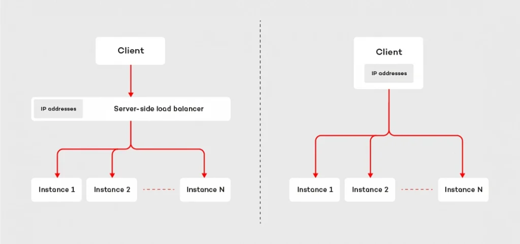
In such a scenario, at least two instances of each microservice are deployed in at least two availability zones. This technique helps our system become resilient and increase its capacity - multiple instances of the microservices are able to handle a significantly higher load. So where is the trick? The redundancy introduces extra complexity. As engineers, we have to ensure that the incoming traffic is spread across all available instances. There are two major techniques which address this problem: server load balancing and client load balancing .

The first approach is based on the assumption that the requester does not know the IP addresses of the responders. Instead of that, the requester communicates with the load balancer, which is responsible for spreading the requests across the microservices connected to it. This design is fairly easy to adopt in the cloud era. IaaS providers usually have built-in, reliable solutions, like Elastic Load Balancer available in Amazon Web Services. Moreover, such a design helps develop routing strategy more sophisticated than plain round ribbon (e.g. adaptive load balancing or chained failover ). The major drawback of this technique is the fact that we have to configure and deploy extra resources, which may be painful if our system consists of hundreds of the microservices. Furthermore, it may affect the latency – each request has extra “network hop” on the load balancer.

The second technique inverts the relation. Instead of a central point used to connect to responders, the requester knows IP addresses of each and every instance of the given microservice. Having such knowledge, the client can choose the responder instance to which it sends the request or opens the connection with. This strategy does not require any extra resources, but we have to ensure that the requester has the IP addresses of all instances of the responder ( see how to deal with it using service discovery pattern ). The main benefit of the client load balancing pattern is its performance – by reduction of one extra “network hop”, we may significantly decrease the latency. This is one of the key reasons why RSocket implements the client load balancing pattern.

Client load balancing in RSocket

On the code level, the implementation of the client load balancing in RSocket is pretty straightforward. The mechanism relies on the LoadBalancedRSocketMono object which works as a bag of available RSocket instances, provided by RSocket supplier. To access RSockets we have to subscribe to the LoadBalancedRSocketMono which onNext signal emits fully-fledged RSocket instance. Moreover, it calculates statistics for each RSocket, so that it is able to estimate the load of each instance and based on that choose the one with the best performance at the given point of time.

The algorithm takes into account multiple parameters like latency, number of maintained connections as well as a number of pending requests. The health of each RSocket is reflected by the availability parameter – which takes values from 0 to 1, where 0 indicates that the given instance cannot handle any requests and 1 is assigned to fully operational socket. The code snippet below shows the very basic example of the load-balanced RSocket, which connects to three different instances of the responder and executes 100 requests. Each time it picks up RSocket from the LoadBalancedRSocketMono object.

@Slf4j

public class LoadBalancedClient {



static final int[] PORTS = new int[]{7000, 7001, 7002};



public static void main(String[] args) {



List rsocketSuppliers = Arrays.stream(PORTS)

.mapToObj(port -> new RSocketSupplier(() -> RSocketFactory.connect()

.transport(TcpClientTransport.create(HOST, port))

.start()))

.collect(Collectors.toList());



LoadBalancedRSocketMono balancer = LoadBalancedRSocketMono.create((Publisher>) s -> {

s.onNext(rsocketSuppliers);

s.onComplete();

});



Flux.range(0, 100)

.flatMap(i -> balancer)

.doOnNext(rSocket -> rSocket.requestResponse(DefaultPayload.create("test-request")).block())

.blockLast();

}



}

It is worth noting, that client load balancer in RSocket deals with dead connections as well. If any of the RSocket instances registered in the LoadBalancedRSocketMono stop responding, the mechanism will automatically try to reconnect. By default, it will execute 5 attempts, in 25 seconds. If it does not succeed, the given RSocket will be removed from the pool of available connections. Such design combines the advantages of the server-side load balancing with low latency and reduction of “network hops” of the client load balancing.

Dead connections & resumabilty mechanism

The question which may arise in the context of dead connections is: what will happen if I have an only single instance of the responder and the connection drops due to network issues. Is there anything we can do with this? Fortunately, RSocket has built-in resumability mechanism.

To clarify the concept let’s consider the following example. We are building an IoT platform which connects to multiple temperature sensors located in different places. Most of them in the distance to the nearest buildings and internet connection sources. Therefore, the devices connect to cloud services using GPRS. The business requirement for our system is that we need to collect temperature readings every second in the real-time, and we cannot lose any data.

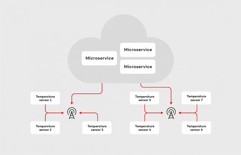
In case of the machine-to-the machine communication within the cloud, streaming data in real-time is not a big deal, but if we consider IoT devices located in areas without access to a stable, reliable internet connection, the problem becomes more complex. We can easily identify two major issues we may face in such a system: the network latency and connection stability . From a software perspective, there is not much we can do with the first one, but we can try to deal with the latter. Let’s tackle the problem with RSocket, starting with picking up the proper interaction model . The most suitable in this case is request stream method, where the microservice deployed in the cloud is the requester and temperature sensor is the responder. After choosing the interaction model we apply resumability mechanism. In RSocket, we do it by method resume() invoked on the RSocketFactory , as shown in the examples below:

@Slf4j

public class ResumableRequester {



private static final int CLIENT_PORT = 7001;



public static void main(String[] args) {

RSocket socket = RSocketFactory.connect()

.resume()

.resumeSessionDuration(RESUME_SESSION_DURATION)

.transport(TcpClientTransport.create(HOST, CLIENT_PORT))

.start()

.block();

socket.requestStream(DefaultPayload.create("dummy"))

.map(payload -> {

log.info("Received data: [{}]", payload.getDataUtf8());

return payload;

})

.blockLast();



}

}

@Slf4j

public class ResumableResponder {



private static final int SERVER_PORT = 7000;

static final String HOST = "localhost";

static final Duration RESUME_SESSION_DURATION = Duration.ofSeconds(60);





public static void main(String[] args) throws InterruptedException {



RSocketFactory.receive()

.resume()

.resumeSessionDuration(RESUME_SESSION_DURATION)

.acceptor((setup, sendingSocket) -> Mono.just(new AbstractRSocket() {

@Override

public Flux requestStream(Payload payload) {

log.info("Received 'requestStream' request with payload: [{}]", payload.getDataUtf8());

return Flux.interval(Duration.ofMillis(1000))

.map(t -> DefaultPayload.create(t.toString()));

}

}))

.transport(TcpServerTransport.create(HOST, SERVER_PORT))

.start()

.subscribe();

log.info("Server running");



Thread.currentThread().join();

}



}

• Please notice that to run provided examples, you need ‘socat’ installed on your machine, please see README file for more details

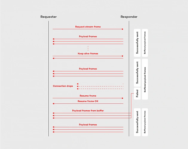
The mechanism on the requester and responder side works similarly, it is based on a few components. First of all, there is a ResumableFramesStore which works as a buffer for the frames. By default, it stores them in the memory, but we can easily adjust it to our needs by implementing the ResumableFramesStore interface (e.g. store the frames in the distributed cache, like Redis). The store saves the data emitted between keep alive frames, which are sent back and forth periodically and indicates, if the connection between the peers is stable. Moreover, the keep alive frame contains the token, which determines Last received position for the requester and the responder. When the peer wants to resume the connection, it sends the resume frame with an implied position . The implied position is calculated from last received position (is the same value we have seen in the Keep Alive frame) plus the length of the frames received from that moment. This algorithm is applied to both parties of the communication, in the resume frame is it reflected by last received server position and first client available position tokens. The whole flow for resume operation is shown in the diagram below:

By adopting the resumability mechanism built in the RSocket protocol, with the relatively low effort we can reduce the impact of the network issues. Like shown in the example above, the resumability might be extremely useful in the data streaming applications, especially in the case of the device to the cloud communication.

Summary

In this article, we discussed more advanced features of the RSocket protocol, which are helpful in reducing the impact of the network on the system operationality. We covered the implementation of the client load balancing pattern and resumability mechanism. These features, combined with the robust interaction model constitutes the core of the protocol.

In the last article of this mini-series , we will cover available abstraction layers on top of the RSocket.

• Please notice that fully working examples are provided here →

DevOps is moving forward and influences various industries, changing the way companies of all sizes deliver software. Few times a year, the community of DevOps experts and practitioners gathers at a conference to discuss the latest trends, share insights, and exchange best practices. This year’s DevOps Enterprise Summit in London was one of these unique chances to participate in this uplifting movement.

When our team got back after DevOps Enterprise Summit in London, we set an engaging, internal discussion. It’s probably a common attitude for every company valuing knowledge exchange, that once attending some interesting conference, your representatives share insights, their thoughts, and news regarding the topics covered during the event. The discussion arose when members of our team had started sharing their takeaways regarding keynotes, speeches, and ideas presented at the conference.

That opened the stream of news and opinions shared by those of our teammates who also follow the latest trends in the industry by attending various meetups, listening to podcasts, etc. Here is the list of the main topics.

DevOps 2nd day – introduction

DevOps is no longer one of these innovative ideas for early adopters, which everyone has heard about but is not aware of how to start with adopting it. Now, it’s a must-have for every organization that intends to stay relevant in competitive markets. When you ask enterprises about using DevOps in their organizations, their representatives will tell you that they have already implemented this culture or are in the process of doing that. On the other hand, if you ask them if they are already satisfied with the adoption, the answer would be no – there are so many practices and principles, what makes the process demanding and it lasts a while.

Nowadays, discussions from “How to implement DevOps in our organization” have evolved into “How can we improve our DevOps practices.” The truth has been told - tech advanced companies need this agile culture to build a successful business. But simultaneously, once they introduce DevOps to their teams, new challenges occur. It’s a natural way of technology/culture adoption. As a person responsible for the cultural shift, you have to communicate it clearly – DevOps wouldn’t solve all your issues. In some cases, it may seem like a reason for some new struggles. The answer to these concerns is simple, your organization is growing, evolution is never done, and change is a constant way of managing things.

Facing DevOps 2nd Day issues is rather the rich man’s problem – you should be there, and you have to tackle them. All the new challenges appear after making an advanced step forward.

Scaling Up - from a core tech team to the entire organization working globally

Core tech teams are the first to adopt the newest solutions, but they cannot work properly without supportive teams (HR, Sales, Marketing, Accounting, etc.). After going through the successful implementation, the next step is to encourage cooperating teams to this mindset and ways of running projects.

As the enterprises that consist of thousands of employees and hundreds of teams cannot provide their crew with the flexibility in designing their very own working culture, there is a need to encourage all teams to once implemented practices.

For tech leaders, responsible for introducing DevOps in their teams, it means that their job evolves to being a DevOps advocate, who presents its value to the whole organizations and makes it a commonly known and used approach. The larger the company is the more complex the entire change becomes, but it's unavoidable when you intend to get the most out of it.

Along with advocating for expanding DevOps in the entire organization, also the very challenging job is to determine the right tech stack. New tools come and go, being responsible for selecting to the most useful toolset that will be in use for a significant period is tough and requires overall knowledge, strategy, and deep understanding of tech processes. Once determined toolset should be recommended to cooperating teams and that may provoke new issues, but is unavoidable. Should you leverage the same tech stack for all teams? When is the right time to adopt new tools? Should you leave it all to the team? Well, there is no right answer to any of these questions, and it highly depends on the situation.

DevOps is changing various industries and not limit itself to tech companies

Attending DOES in London was a great opportunity to learn more about how DevOps influences the world’s coolest companies, not often associated with technology. Let’s look at the two of the most recognized sportswear retailers - Adidas and Nike. Both these brands are synonyms to heroism, activity, sports achievements. But, as their representatives presented, both companies can overshadow many of tech brands, with their DevOps maturity and advanced approach to using technology in growing their businesses.

Following these business cases, we can agree that the time when cutting-edge technologies and methodologies often paired with them are limited to IT companies is officially over. Nowadays, industry by industry is convincing themselves to the latest solutions as developing software for internal processes is a natural competitive advantage.

Continuous adaptation and life-long learning

The best thing about working in a DevOps culture is that you just cannot say that the process has finished, that a company has transformed, and that a team has mastered the way of delivering software. Taking into account how creative the community gathered around DevOps is, how fast new ideas arise, how often its fundamentals are improved, you have to keep learning about new things.

It would be extremely comfortable if a company could once undergo digital transformation and treat the process as a completed. But if we take a look at the evolution of technology and methodologies designed to take full advantage of its capabilities, it’s obvious that it cannot be finished. Adoption of a DevOps mindset is the beginning of a change and should be conducted as a never-ending evolution.

You can’t be good at everything, which is fine, but you have to know your pain points

Excluding enterprises with enormous budgets, all organizations have limitations that obligate them to focus only on some aspects of conducting business processes. As an expert, a professional who works in a highly competitive market, you have to follow the latest trends, be aware of upcoming solutions, and cutting-edge technologies that are reshaping the business.

Being up to date is extremely important, but almost equally essential is the ability to decide on which things you cannot engage, as your time and resources are not flexible. Being responsible for your company means being aware of pain points and focusing only on the things that matter. Technology is developing extremely fast, you cannot afford to be an early adopter of every promising solution. Your job is to make responsible decisions, based on your deep understanding of the current state of technology development.

If you don’t know what to choose, think about what’s better for your business

DevOps came to being as an efficient solution to the common challenge - how to sync software development and IT operations processes to help companies thrive. Built with business effectiveness in mind, this culture has the right foundations. Choosing approaches that were designed to resolve not only internal issues but also to enable revenue growth is good for your overall success.

Anytime you face a situation when you have to decide between different solutions, always consider your company's long term perspective. When you are focused only on your goals, you may contribute to building siloses. The key to determine which ideas are the right to choose is their overall usability. We all, as professionals in our niches, may tend to prefer idealistic solutions. It’s important that we don’t work in an ideal world and our job is verified by the market.

Adopting new tools and technologies is challenging, but the real quest appears when it comes to change people's habits and company culture

If you want to make your colleagues angry, implement new toolset and new technologies in your team. Apart from tech freaks and beta testers, people are rather skeptical when it comes to learning new features and new UI. Things change when you provide them with solutions that make their work easier and more efficient.

But the real trouble occurs when you are trying to change your company's culture. It’s nothing new that we protect what we know, don’t want to change our habits, or even feel in danger when someone is trying to reshape the way we have been doing our job for ages. Your colleagues defend themselves which is natural, you cannot change it. You have to take this into account and make sure that the process will be smooth enough to help everyone adjust to the new reality. Start with small steps, be the example, discuss the issues, and explain potential opportunities. Shock therapy as a path to the cultural shift is not the way to go.

As a team developing our product -  Cloudboostr - multicloud, enterprise-ready Kubernetes, we help companies adopt a complete cloud-native stack, built with proven patterns and best practices, so they could focus their resources on improving their working culture. The feedback we’re receiving is that our customer’s teams are more open to start using new toolset then to change the approach to software delivery.

Being a DevOps Pprofessional is hot now

DevOps practitioners are much in demand. It’s a great time to master the skills required to be a specialist in DevOps as companies of all sizes are looking for help in modernizing their businesses. There are various ways of approaching it - by building an in-house team, outsourcing processes, collaborating with external consultants. Companies choose preferred manner accordingly to their needs and budget.

No matter if you work in a dedicated team at a huge enterprise, developing startup with your colleagues, or providing consulting services for global brands, being a DevOps expert is a strong competitive advantage on the talent market.

DOES London - sum up

DevOps is moving forward and is great to be among teams that contribute to its evolution. We are willing to  share our expertise , exchange knowledge, and learn from the best in the business, and conferences like DevOps Enterprise Summit are the best platforms to do it.

This article is the first one of the mini-series which will help you to get familiar with RSocket – a new binary protocol which may revolutionize machine-to-machine communication. In the following paragraphs, we discuss the problems of the distributed systems and explain how these issues may be solved with RSocket. We focus on the communication between microservices and the interaction model of RSocket.

• Please notice that code examples presented in the article are available on GitHub →

Communication problem in distributed systems

Microservices are everywhere, literally everywhere. We went through the long journey from the monolithic applications, which were terrible to deploy and maintain, to the fully distributed, tiny, scalable microservices. Such architecture design has many benefits; however, it also has drawbacks, worth mentioning. Firstly, to deliver value to the end customers, services have to exchange tons of data. In the monolithic application that was not an issue, as the entire communication occurred within a single JVM. In the microservice architecture, where services are deployed in the separate containers and communicate via an internal or external network, networking is a first-class citizen. Things get more complicated if you decide to run your applications in the cloud, where network issues and periods of increased latency is something you cannot fully avoid. Rather than trying to fix network issues, it is better to make your architecture resilient and fully operational even during a turbulent time.

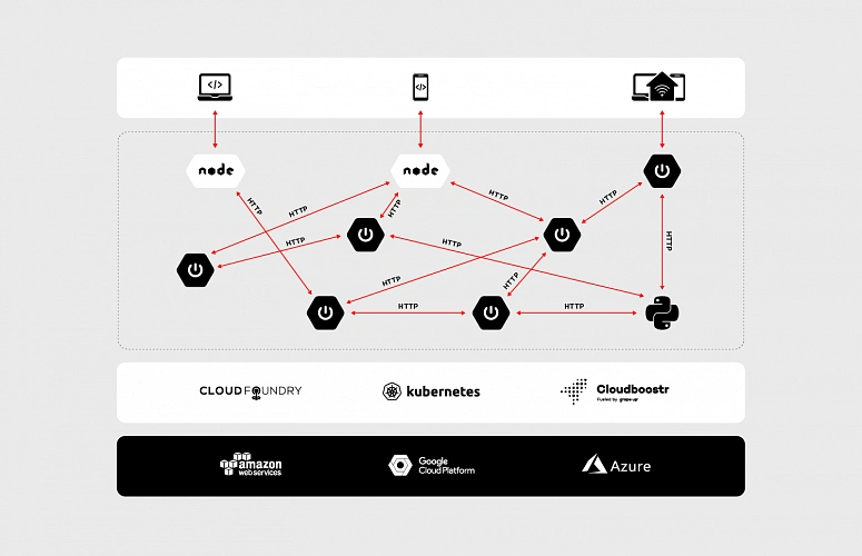
Let’s dive a bit deeper into the concept of the microservices, data, communication and the cloud. As an example, we will discuss the enterprise-grade system which is accessible through a website and mobile app as well as communicates with small, external devices (e.g home heater controller). The system consists of multiple microservices, mostly written in Java and it has a few Python and node.js components. Obviously, all of them are replicated across multiple availability zones to assure that the whole system is highly available.

To be IaaS provider agnostic and improve developer experience the applications are running on top of PaaS. We have a wide range of possibilities here: Cloud Foundry, Kubernetes or both combined in Cloudboostr are suitable. In terms of communication between services, the design is simple. Each component exposes plain REST APIs – as shown in the diagram below.

At first glance, such an architecture does not look bad. Components are separated and run in the cloud – what could go wrong? Actually, there are two major issues – both of them related to communication.

The first problem is the request/response interaction model of HTTP. While it has a lot of use cases, it was not designed for machine to machine communication. It is not uncommon for the microservice to send some data to another component without taking care about the result of the operation (fire and forget) or stream data automatically when it becomes available (data streaming). These communication patterns are hard to achieve in an elegant, efficient way using a request/response interaction model. Even performing simple fire and forget operation has side effects – the server has to send a response back to the client, even if the client is not interested in processing it.

The second problem is the performance. Let’s assume that our system is massively used by the customers, the traffic increases, and we have noticed that we are struggling to handle more than a few hundred requests per second. Thanks to the containers and the cloud, we are able to scale up our services with ease. However, if we track resource consumption a bit more, we will notice that while we are running out of memory, the CPUs of our VMs are almost idle. The issue comes from the thread per request model usually used with HTTP 1.x, where every single request has its own stack memory. In such a scenario, we can leverage the reactive programming model and non-blocking IO. It will significantly cut down memory usage, nevertheless, it will not reduce the latency. HTTP 1.x is a text-based protocol thus size of data that need to be transferred is significantly higher than in the case of binary protocols.

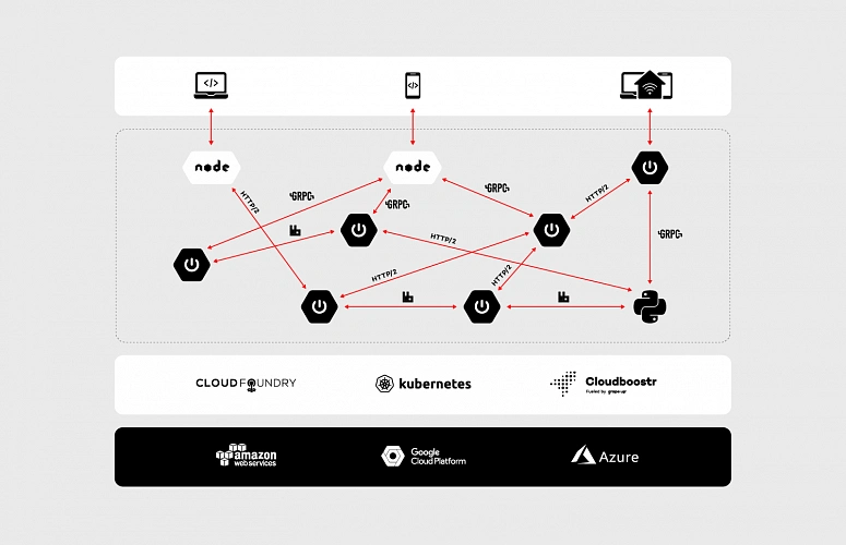
In the machine to machine communication we should not limit ourselves to HTTP (especially 1.x), its request/response interaction model and poor performance. There are many more suitable and robust solutions out there (on the market). Messaging based on the RabbitMQ, gRPC or even HTTP 2 with its support for multiplexing and binarized payloads will do way better in terms of performance and efficiency than plain HTTP 1.x.

Using multiple protocols allow us to link the microservices in the most efficient and suitable way in a given scenario. However, the adoption of multiple protocols forces us to reinvent the wheel again and again. We have to enrich our data with extra information related to security and create multiple adapters which handle translation between protocols. In some cases, transportation requires external resources (brokers, services, etc.) which need to be highly available. Extra resources entail extra costs, even though all we need is simple, message-based fire and forget operation. Besides, a multitude of different protocols may introduce serious problems related to application management, especially if our system consists of hundreds of microservices.

The issues mentioned above are the core reasons why RSocket was invented and why it may revolutionize communication in the cloud. By its reactiveness and built-in robust interaction model, RSocket may be applied in various business scenarios and eventually unify the communication patterns that we use in the distributed systems.

RSocket to the rescue

RSocket is a new, message-driven, binary protocol which standardizes the approach to communication in the cloud. It helps to resolve common application concerns with a consistent manner as well as it has support for multiple languages (e.g java, js, python) and transport layers (TCP, WebSocket, Aeron).
In the following sections, we will dive deeper into protocol internals and discuss the interaction model.

Framed and message-driven

Interaction in RSocket is broken down into frames. Each frame consists of a frame header which contains the stream id, frame type definition and other data specific to the frame type. The frame header is followed by meta-data and payload – these parts carry data specified by the user.

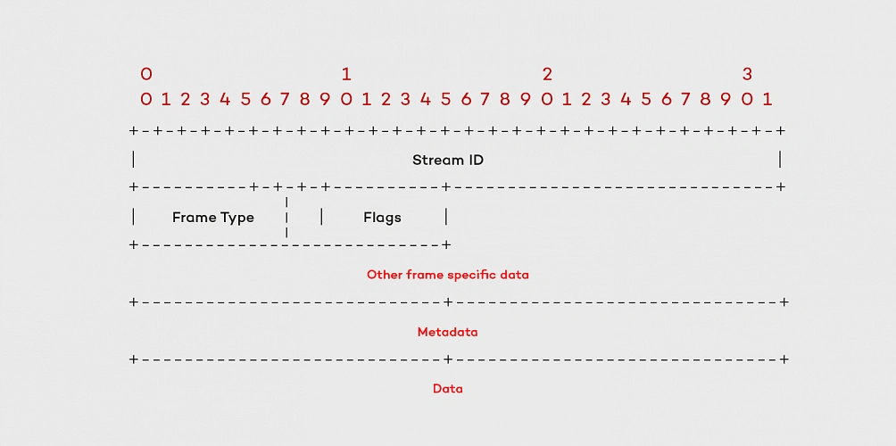
There are multiple types of frames which represent different actions and available methods of the interaction model. We’re not going to cover all of them as they are extensively described in the official documentation (http://rsocket.io/docs/Protocol). Nevertheless, there are few which are worth noting. One of them is the Setup Frame which the client sends to the server at the very beginning of the communication. This frame can be customized so that you can add your own security rules or other information required during connection initialization. It should be noted that RSocket does not distinguish between the client and the server after the connection setup phase. Each side can start sending the data to the other one – it makes the protocol almost entirely symmetrical.

Performance

The frames are sent as a stream of bytes. It makes RSocket way more efficient than typical text-based protocols. From a developer perspective, it is easier to debug a system while JSONs are flying back and forth through the network, but the impact on the performance makes such convenience questionable. The protocol does not impose any specific serialization/deserialization mechanism, it considers the frame as a bag of bits which could be converted to anything. That makes possible to use JSON serialization or more efficient solutions like Protobuf or AVRO.

The second factor, which has a huge impact on RSocket performance is the multiplexing. The protocol creates logical streams (channels) on the top of the single physical connection. Each stream has its unique ID which, to some extent, can be interpreted as a queue we know from messaging systems. Such design deals with major issues known from HTTP 1.x – connection per request model and weak performance of “pipelining”. Moreover, RSocket natively supports transferring of the large payloads. In such a scenario the payload frame is split into several frames with an extra flag – the ordinal number of the given fragment.

Reactiveness & Flow Control

RSocket protocol fully embraces the principles stated in the Reactive Manifesto . Its asynchronous character and thrift in terms of the resources helps decrease the latency experienced by the end users and costs of the infrastructure. Thanks to streaming we don’t need to pull data from one service to another, instead, the data is pushed when it becomes available. It is an extremely powerful mechanism, but it might be risky as well. Let’s consider a simple scenario: in our system, we are streaming events from service A to service B. The action performed on the receiver side is non-trivial and require some computation time. If service A pushes events faster than B is able to process them, eventually, B will run out of resources – the sender will kill the receiver. Since RSocket uses the reactor, it has built-in support for the flow control , which helps to avoid such situations.

We can easily provide the backpressure mechanism implementation, adjusted to our needs. The receiver can specify how much data it would like to consume and will not get more than that until it notifies the sender that it is ready to process more. On the other hand, to limit the number of incoming frames from the requester, RSocket implements a lease mechanism. The responder can specify how many requests requester may send within a defined time frame.

The API

As mentioned in the previous section, RSocket uses Reactor, so that on the API level we are mainly operating on Mono and Flux objects. It has full support for reactive signals as well – we can easily implement “reaction” on different events – onNext, onError, onClose, etc.

The following paragraphs will cover the API and each and every interaction option available in RSocket. The discussion will be backed with the code snippets and the description for all the examples. Before we jump into the interaction model, it is worth describing the API basics, as it will come up in the multiple code examples.

Setting up the connection with RSocketFactory

Setting up the RSocket connection between the peers is fairly easy. The API provides factory (RSocketFactory) with factory methods receive and connect to create RSocket and CloseableChannel instances on the client and the server side respectively. Second common property present in both parties of the communication (the requester and the responder) is a transport. RSocket can use multiple solutions as a transport layer (TCP, WebSocket, Aeron). Whichever you choose the API provides the factory methods which allows you to tweak and tune the connection.

RSocketFactory.receive()

.acceptor(new HelloWorldSocketAcceptor())

.transport(TcpServerTransport.create(HOST, PORT))

.start()

.subscribe();

RSocketFactory.connect()

.transport(TcpClientTransport.create(HOST, PORT))

.start()

.subscribe();

Moreover, in the case of the responder, we have to create a socket acceptor instance. The SocketAcceptor is an interface which provides the contract between the peers. It has a single method accept which accepts the RSocket for sending requests and returns an instance of RSocket that will be used for handling the requests from the peer. Besides providing the contract the SocketAcceptor enables us to access the setup frame content. On the API level, it is reflected by ConnectionSetupPayload object.

public interface SocketAcceptor {

Mono<RSocket> accept(ConnectionSetupPayload setup, RSocket sendingSocket);

}

As shown above, setting up the connection between the peers is relatively easy, especially for those of you who worked with WebSockets previously – in terms of the API both solutions are quite similar.

Interaction model

After setting up the connection we are able to move on to the interaction model. RSocket supports following operations:

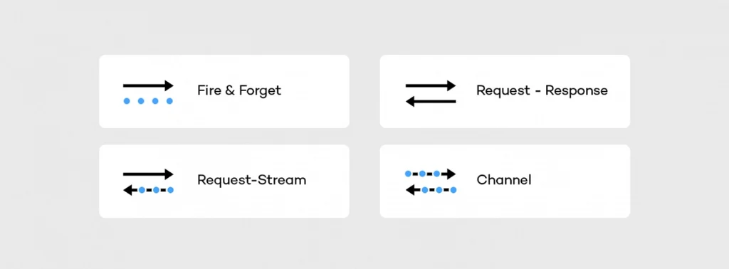
The fire and forget , as well as the metadata push , were designed to push the data from the sender to the receiver. In both scenarios the sender does not care about the result of the operation – it is reflected on API level in a return type (Mono). The difference between these actions sits in the frame. In case of fire and forget the fully-fledged frame is sent to the receiver, while for the metadata push action the frame does not have payload – it consists only of the header and the metadata. Such a lightweight message can be useful in sending notifications to the mobile or peer-to-peer communication of IoT devices.

RSocket is also able to mimic HTTP behavior. It has support for request-response semantics, and probably that will be the main type of interaction you are going to use with RSocket. In streams context, such an operation can be represented as a stream which consists of the single object. In this scenario, the client is waiting for the response frame, but it does it in a fully non-blocking manner.

More interesting in the cloud applications are the request stream and the request channel interactions which operate on the streams of data, usually infinite. In case of the request stream operation, the requester sends a single frame to the responder and gets back the stream of data. Such interaction method enables services to switch from the pull data to the push data strategy. Instead of sending periodical requests to the responder requester can subscribe to the stream and react on the incoming data – it will arrive automatically when it becomes available.

Thanks to the multiplexing and the bi-directional data transfer support, we can go a step further using the request channel method. RSocket is able to stream the data from the requester to the responder and the other way around using a single physical connection. Such interaction may be useful when the requester updates the subscription – for example, to change the subscription criteria. Without the bi-directional channel, the client would have to cancel the stream and re-request it with the new parameters.

In the API, all operations of the interaction model are represented by methods of RSocket interface shown below.

public interface RSocket extends Availability, Closeable {



Mono<Void> fireAndForget(Payload payload);



Mono<Payload> requestResponse(Payload payload);



Flux<Payload> requestStream(Payload payload);



Flux<Payload> requestChannel(Publisher<Payload> payloads);



Mono<Void> metadataPush(Payload payload);



}

To improve the developer experience and avoid the necessity of implementing every single method of the RSocket interface, the API provides abstract AbstractRSocket we can extend. By putting the SocketAcceptor and the AbstractRSocket together, we get the server-side implementation, which in the basic scenario may look like this:

@Slf4j

public class HelloWorldSocketAcceptor implements SocketAcceptor {



@Override

public Mono<RSocket> accept(ConnectionSetupPayload setup, RSocket sendingSocket) {

log.info("Received connection with setup payload: [{}] and meta-data: [{}]", setup.getDataUtf8(), setup.getMetadataUtf8());

return Mono.just(new AbstractRSocket() {

@Override

public Mono<Void> fireAndForget(Payload payload) {

log.info("Received 'fire-and-forget' request with payload: [{}]", payload.getDataUtf8());

return Mono.empty();

}



@Override

public Mono<Payload> requestResponse(Payload payload) {

log.info("Received 'request response' request with payload: [{}] ", payload.getDataUtf8());

return Mono.just(DefaultPayload.create("Hello " + payload.getDataUtf8()));

}



@Override

public Flux<Payload> requestStream(Payload payload) {

log.info("Received 'request stream' request with payload: [{}] ", payload.getDataUtf8());

return Flux.interval(Duration.ofMillis(1000))

.map(time -> DefaultPayload.create("Hello " + payload.getDataUtf8() + " @ " + Instant.now()));

}



@Override

public Flux<Payload> requestChannel(Publisher<Payload> payloads) {

return Flux.from(payloads)

.doOnNext(payload -> {

log.info("Received payload: [{}]", payload.getDataUtf8());

})

.map(payload -> DefaultPayload.create("Hello " + payload.getDataUtf8() + " @ " + Instant.now()))

.subscribeOn(Schedulers.parallel());

}



@Override

public Mono<Void> metadataPush(Payload payload) {

log.info("Received 'metadata push' request with metadata: [{}]", payload.getMetadataUtf8());

return Mono.empty();

}

});

}

}

On the sender side using the interaction model is pretty simple, all we need to do is invoke a particular method on the RSocket instance we have created using RSocketFactory, e.g.

socket.fireAndForget(DefaultPayload.create("Hello world!"));

• For more examples of the methods available in the RSocket interaction model please visit GitHub →

More interesting on the sender side is the implementation of the backpressure mechanism. Let’s consider the following example of the requester side implementation:

public class RequestStream {



public static void main(String[] args) {



RSocket socket = RSocketFactory.connect()

.transport(TcpClientTransport.create(HOST, PORT))

.start()

.block();

socket.requestStream(DefaultPayload.create("Jenny", "example-metadata"))

.subscribe(new BackPressureSubscriber());



socket.dispose();

}



@Slf4j

private static class BackPressureSubscriber implements Subscriber<Payload> {



private static final Integer NUMBER_OF_REQUESTED_ITEMS = 5;

private Subscription subscription;

int receivedItems;



@Override

public void onSubscribe(Subscription s) {

this.subscription = s;

subscription.request(NUMBER_OF_REQUESTED_ITEMS);

}



@Override

public void onNext(Payload payload) {

receivedItems++;

if (receivedItems % NUMBER_OF_REQUESTED_ITEMS == 0) {

log.info("Requesting next [{}] elements", NUMBER_OF_REQUESTED_ITEMS);

subscription.request(NUMBER_OF_REQUESTED_ITEMS);

}

}



@Override

public void onError(Throwable t) {

log.error("Stream subscription error [{}]", t);

}



@Override

public void onComplete() {

log.info("Completing subscription");

}

}



}

In this example, we are requesting the stream of data, but to ensure that the incoming frames will not kill the requester we have the backpressure mechanism put in place. To implement this mechanism we use request_n frame which on the API level is reflected by the subscription.request(n) method. At the beginning of the subscription [ onSubscribe(Subscription s) ], we are requesting 5 objects, then we are counting received items in onNext(Payload payload). When all expected frames arrived to the requester, we are requesting the next 5 objects – again using subscription.request(n) method. The flow of this subscriber is shown in the diagram below:

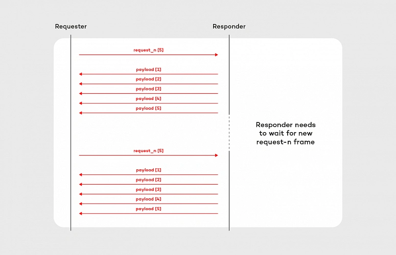
Implementation of the backpressure mechanism presented in this section is very basic. In the production, we should provide a more sophisticated solution based on more accurate metrics e.g. predicted/average time of computation. After all, the backpressure mechanism does not make the problem of an overproducing responder disappear. It shifts the issue to the responder side, where it can be handled better. Further reading about backpressure is available here on Medium and here on GitHub .

Summary

In this article, we discuss the communication issues in the microservice architecture, and how these problems can be solved using RSocket. We covered its API and the interaction model backed with simple “hello world” example and basic backpressure mechanism implementation.

In the next articles of this series, we will cover more advanced features of RSocket including Load Balancing and Resumability as well as we will discuss abstraction over RSocke t – RPC and Spring Reactor.

• Please notice that fully working examples are provided here →

With ever-growing IT projects, automation is nowadays a must-have. From building source code and testing to versioning and deploying, CI/CD tools were always the anonymous team member, who did the job no developer was eager to do. Today, we will take a look at some tips regarding one of the newest tools - Concourse CI. First, we will speed up our Concourse jobs, then we’ll ease the development of the new pipelines for our projects.

Aggregate your steps

By default, Concourse tasks in a job are executed separately. This is perfectly fine for small Concourse jobs that last a minute or two. It also works well at the beginning of the project, as we just want to get the process running. But at some point, it would be nice to optimize our builds.

The simplest way to save time is to start using the aggregate keyword. It runs all the steps declared inside of it in parallel. This leads to time-savings in both - script logic execution and in the overhead that occurs when starting the next task.

Neat, so where can we use it? There are 2 main parts of a job where the aggregation is useful:

1. Resource download and upload.
2. Tests execution.

Get and put statements are ideal targets because download and upload of resources are usually completely independent. Integration tests, contract tests, dependency vulnerabilities tests, and alike are also likely candidates if they don’t interfere with one another. Project build tasks? Probably not, because those are usually sequential and we require their output to proceed.

How much time can aggregating save? Of course, it depends. Assuming we can’t aggregate steps that build and test our code, we do get the advantage of simultaneous upload and download of our resources as well as we get less visible step-to-step overhead. We usually save up to two, maybe even three minutes. The largest saving we got was from over half an hour to below ten minutes. Most of the saved time came from running test-related tasks in parallel.

Use docker images with built-in tools

This improvement is trickier to implement but yields a noticeable build time gains. Each task runs in a container, and the image for that container has a certain set of tools available. At some point in the project comes a time where no available image has the tool required. First thing developers do is they download that tool manually or install it using a package manager as a part of the task execution. This means that the tool is fetched every time the task runs. On top of that, the console output is flooded with tool installation logs.

The solution is to prepare a custom container image that already has everything needed for a task to complete. This requires some knowledge not directly related to Concourse, but for example to Docker. With a short dockerfile and a couple of terminal commands, we get an image with the tools we need.

1. Create dockerfile.
2. Inside of the file, install or copy your tools using RUN or COPY commands.
3. Build the image using docker build.
4. Tag and push the image to the registry.
5. Change image_resource part in your Concourse task to use the new image.

That’s it, no more waiting for tools to install each time! We could even create a pipeline to build and push the image for us.

Create pipelines from a template

Moving from time-saving measures to developer convenience tips, here’s one for bigger projects. Those usually have a certain set of similar build pipelines with the only differences being credentials, service names, etc. - parameters that are not hardcoded in the pipeline script and are injected at execution time from a source like CredHub. This is typical for Cloud Foundry and Kubernetes web projects with microservices. With a little bit of creativity, we could get a bash or python script to generate those pipelines from a single template file.

First, we need to have a template file. Take one of your existing pipeline specifications and substitute parameter names with their pipeline agnostic version. Our script needs to loop over a pipeline names list, substitute generic parameter names with proper pipeline related ones that are available in Credhub and then set the pipeline in Concourse with the fly CLI.

The second part of the equation here is a Concourse job that watches for changes in the template file in a Git repository and starts the pipeline generation script. With this solution, we have to change only one file to get all pipelines updated, and on top of that, a commit to pipeline repository is sufficient to trigger the update.

Log into a task container to debug issues

When debugging Concourse task failures, the main source of information on failure is the console. A quick glance at the output is enough to solve most of the problems. Other issues may require a quick peek into the environment of an unsuccessful task. We can do that with fly intercept command.

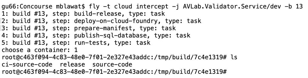
Fly intercept allows us to log into a container that executed a specific task in a specific job run. Inside we can see the state of the container when task finished and can try to find the root of failure. There may be an empty environment variable - we forgot to set the proper param in a yml file. The resource has a different structure inside of it - we need to change the task script or the resource structure. When the work is done, don’t forget to log out of the container. Oh, and don’t wait too long! Those containers can be disposed of by Concourse at any time.

Use Visual Studio Code Concourse add-on

The last thing I want to talk about is the Concourse CI Pipeline Editor for Visual Studio Code. It’s a plugin that offers suggestions, documentation popups, and error checking for Concourse yml files. If you use the pipeline template and generation task from the previous tip, then any syntax error in your template will be discovered as late as the update task updating the pipelines from the template. That’s because you won’t run fly set-pipeline yourself. Fixing such issue requires a new commit in the pipeline repository.

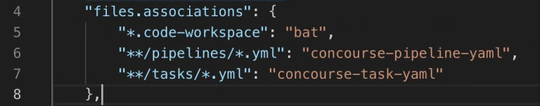
With the plugin, any unused resource or a typo in property name will be detected immediately. Add-on will also help you write new pieces of automation code by suggesting keywords and showing available values for Concourse commands. The only action required is to update the files.associations section in the settings. We use separate directories for pipelines and tasks, so we have set it up as follows:

Conclusion

And that’s it! We hope you have found at least one tip useful and will use it in your project. Aggregate is an easy one to implement, and it’s good to have a habit of aggregating steps from the start. Custom images and pipeline templates are beneficial in bigger projects where they help keep CI less clunky. Finally, fly intercept and the VSC add-on are just extra tools to save time during the pipeline development.

A Sprint Review is a meeting that closes and approves a Sprint in Scrum. The value of this meeting comes to inspect the increment and adapt the Product Backlog accordingly to current business conditions. This is a session where the Scrum Team and all interested stakeholders can attend to exchange information regarding progress made during the Sprint. They discuss problems and update the work plan to meet current market needs and approach a once determined product vision in a new way.

This meeting is supposed to enable feedback loop and foster collaboration, especially between the Scrum Team and all Stakeholders. A Sprint Review will be valuable for product development if there is an overall understanding of its purpose and plan. To maximize its value, it’s good to be aware of the impediments Scrum Team could meet. We would like to share our experience with a Sprint Review, the most important problems and facts discovered during numerous projects run by our team from Grape Up . As one of our company values is Drive Change, we are continuously working on enhancing our Scrum Process by investigating problems, resolving them, and implementing proper solutions to our daily work.

“Meetings – coding work balance.“

It’s a hard reality for managers leading projects. A lot of teams have a problem with too many meetings which disorganize daily work and may be an obstacle to deliver increment. Every group consists of both; people who hate meetings and prefer focusing on coding and meetings-lovers who always have thousands of questions and value teamwork over working independently. Internal team meetings or chats with stakeholders are an important part of daily work only when they bring any benefit to the team or product. Scrum prescribes four meetings during a Sprint: Sprint planning, the Daily Scrum, a Sprint Review and a Sprint Retrospective. It all makes collaboration critical to run a successful Scrum Team.

A stereotype developer who sits in his basement and doesn’t go on the daylight, who is introvert doesn’t fit this vision. Communication skills are very important for every scrum developer. Beyond technical skills and the ability to create good quality code, they need to develop their soft skills. Meetings are time-consuming and here comes a real threat that makes many people angry – after a few quarters of discussions, you may see no progress in coding. You need to confront with opinions of your colleagues and many times it’s not easy. Moreover, you need to describe to the managers what are you doing in a different language than JavaScript or Python.

For many professionals, the ideal world would be to sit comfortably in front of a screen and just write good quality code. But wait… Do people really want to do the work that no one wants? Create functionalities no one needs? Feedback exchange may not help to speed up the production process but for sure can boost the quality and usability of an application. The main idea of Scrum is to inspect and adapt continuously, and there is no way to do it without discussion and collaboration. In agile, the team’s information flow and early transformation is the main thing. It saves money and “lives”!

A Sprint Review gives a unique chance to stop for a moment and look at all the work done. It’s an important meeting that helps to keep roadmap and backlog in good health together with the market expectations. This is not only a one-side demo but a discussion of all participating guests. Each presented story should be talked through. Each attendee can ask questions, and the Product Owner or a team member should be able to answer it. It’s good to be as neutral as it’s possible neither praise nor criticize. Focus on evaluating features, not people.

Our team works for external clients from the USA, and our contact with them is constricted by time zones. A Sprint Review helps us to understand better client needs and step into their shoes. The development team can share their ideas and obstacles, and what is most important, enrich the understanding of the business value of their input. Each team member presents own part of a project, describes how it works, and asks the client for feedback. Sometimes we even share a work that's not 100% completed to be sure we are heading into the right direction to adapt on the early phase of implementation.

"Keep calm and work": No timeboxing

A Sprint Review should be open to everyone interested in joining the discussion. Main guests are the Product Owner, the Development Team, and business representation, but other stakeholders are also welcome. Is there a Scrum Master on board? For sure it should be! This may lead to a quite big meeting when many points of view occur and clash with each other. Uncontrolled discussion lasting hours is a real threat.

The Scrum Master’s role is to keep all meetings on track and allow everyone to talk. Parkinson’s Law is an old adage that says "work expands so as to fill the time available for its completion." Every Scrum Master’s golden rule of conducting meetings should be to schedule session blocks for the minimum amount of time needed. Remember that too long gathering may be a waste of time. Even if you are able to finish a meeting in 30 min, but had planned it for 1 hour, it will finally take the entire hour. Don’t forget that long and worthless meetings are boring.

An efficient Sprint Review needs to keep all guests focused and engaged. For a 1-week sprint, it should last about one hour; for a 2-week sprint, two hours. The Scrum Master’s role is to ensure theses time boxes but also to facilitate a meeting and inform when discussion leaves a trace. There should be time to present the summary of the last sprint: what was done and what wasn’t, to demonstrate progress and to answer all questions. Finally, additional time for gathering new ideas that will for sure appear. The second part of the meeting should be focused on discussing and prioritizing current backlog elements to adjust to customer and market needs. It’s a good moment for all team members to listen to the customer and get to know the management perspective and plan the next release content and date. A Sprint Review is an ideal moment for stakeholders to bring new ideas and priorities to the dev team and reorder backlog with Product Owner. During this session, all three Scrum pillars meet: transparency, inspection, and adaptation.

YOLO! : Preparation is for weak

A good plan is an attribute of a well-conducted meeting! No one likes mysterious meetings. An invitation should inform not only about time, place, and date of the meeting but also about the high-level program. Agenda is the first step of a good Sprint Review but not the only one. To be sure that Sprint Review will be satisfying for all participants, everyone needs to be well prepared. Firstly, the Product Owner should decide what work can be presented and create a clear plan of the demo and the entire meeting. The second step is to determine people responsible for each presented feature. Their job is to prepare the environment, interesting scenarios, and all needed materials. But before asking the team for it, make sure they know how to do it. Not all of the people are born presenters, but they can become one with your help.

In our team, we help each other with preparations to the Sprint Review. We work in Poland, but our customers are mostly from the USA. Not only the distance and time difference is a challenge but also language barriers. If there is a need everyone can ask for a rehearsal demo where we can present our work, discuss potential problems, and ask each other for more details. We’re constantly improving our English to make sure everything is clear to our clients. This boosts everyone’s self-confidence and final receipt. Team members know what to do, they’re ready for potential questions and focus on input from stakeholders. This is how we improve not only Sprint Reviews to be better and better but also communication skills.

"Work on your own terms": No DoD

“How ready is your work?”. Imagine a world where each developer decides when s/he finished work on her/his own terms. For one, it’s when the code is just compiled, for others it includes unit tests and it's compatible with coding standards, or even integration and usability tests. Everything works on a private branch but when it comes to integrating… boom! The team is trying to prepare a version to demonstrate but the final product crashes. The Product Owner and stakeholders are confused. A sprint without potentially releasable work is a wasted sprint. This dark scenario shouldn’t have happened to any Scrum Team.

To save time and to avoid misunderstandings, it’s good to speak the same language. All team members should be aware of the meaning of the word “done”. In our team, this keeps us on track with a transparent view of what work really can be found as delivered in a sprint. Definition of Done is like an examination of consistency for a team. Clear, generally achievable, and easy to understand steps to decide how much work is done to create a potentially releasable feature. This provides all stakeholders with clear information and allows the planning of the next business steps.

It is a guide that dictates when teams can legitimately claim that a given user’s story/task is "done" and can be moved to the next level - approval by the Product Owner and release. Basic elements of our DoD are; the code reviewed by other developers, merged to develop branch, and deployed on DEV/QA environment, and finally properly tested by QA and developers with the manual, and automation tests. The last step comes to fixing all defects, verifying if all the Acceptance Criteria are met, and reviewing by the Product Owner. Only when all DoD elements are done, we surely say that this is something we can potentially release when it will be needed.

"Curiosity killed a cat": don't report progress

Functionalities which meet requirements of Definition of Done are the first candidates to be shared on the Sprint Review. In the ideal Agile World, it’s not recommended to demonstrate not finished work. Everything we want to present should be potentially releasable… but wait! Could you agree that an ideal Agile World doesn’t exist? How many times external clients really don’t know how they want to implement something until they see the prototype.

Our company provides not only product development services but also consulting support. We don’t limit this collaboration to performing tasks, in most cases we co-create applications with our clients, advise the best solutions, and tackle their problems. Many times, there’s is no help from a Graphic Designer or a UX team. That happened to us. That’s why we have improved our Sprint Review. Since then we present not only finished work but also this in progress. Advanced features should be divided into smaller stories which can be delivered during one sprint. Final feature will be ready after a few sprints but completed parts of it should be demonstrated. It helps us discuss the vision and potential obstacles. Each meeting starts with work “done” and goes to work "in progress". What is the value? Clients trust us, believe in our ideas but at the same time still, have final word and control. Very quickly we can find out if we’re moving in the right direction or not. It’s better to hear “I imagined it in a different way, let’s change something” after one sprint than live with the falsified view of reality till the feature release.

"As you make your bed, so you must lie in it": don't inform about obstacle

Finally, even the best and ideal team can turn into the worst bunch of co-workers if they are not honest. We all know that customer satisfaction is a priority but not at all costs. It is not a shame to talk about problems the team met during the Sprint or obstacles we face with advanced features. Stakeholders need to know clearly the state of product development to confront it with the business teams involved in a project; marketing, sales or colleagues responsible for the project budget. When tasks take much more time than predicted, it’s better to show a delay in production and explain their reasons. Putting lipstick on a pig does not work. Transparency, which is so important is Scrum, allows all the people involved in the project to make good decisions for further product development. A Product Owner, as someone who defines the product vision, evaluates product progress and anticipates client needs, is obligated to look at the entire project from a general perspective, and monitor its health.

One more time, a stay-cool rule is up to date. Don’t panic and share a clear message based on facts.

We all want to implement the best practices and visions that make our life and work more productive and fruitful. Scrum helps with its values, pillars, and rules . But there is a long way from unconscious incompetence to conscious competence. It’s good to be aware of the problems we can meet and how to manage with them. “Rome wasn't built in a day”. If your team doesn’t use a Sprint Review but only a demo at the end of the sprint, just try to change it. As a team member, Scrum Master or Product Owner, observe, analyze and adapt continuously not only with your product but also with your team and processes.

Pro Tips:

• Adjust the time of a Sprint Review to accurate needs. For a 1-week Sprint, it’s one hour, for a 2-week Sprint give it two hours. It is a recommendation based on our experience.
• Have a plan. Create stable agenda and a brief summary of a Sprint and share it before meeting with everyone invited to a Sprint Review.
• Prepare yourself and a team. Coach your team members and discuss potential questions that can be asked by stakeholders.
• Facilitate meeting to keep all stakeholders interested and give everyone possibility to share feedback.
• Create a clear Definition of Done that is understandable by all team members and stakeholders.
• Be honest. Talk about problems and obstacles, show work in progress if you see there is value in it. Engage and co-create the product with your client.
• Try to be as neutral as it’s possible nor to praise or criticize. Focus on facts and substantive information.

We know that adjusting to the new working environment may be tough. It’s even more challenging when you have to collaborate with people located in different offices around the world. We both experienced such a demanding situation and want to describe a few problems and suggest some ways to tackle them. We hope to help fellow professionals who are at the beginning of this ambitious career path. In this article, we want to elaborate on working in multicultural, half-remote teams and main challenges related to this. To dispel doubts, by “half remote team” we mean a situation in which part of the group works together on-site when other part/parts of the crew work in other places, single or in a larger group/groups. We've gathered our experiences during our works in this kind of teams in Europe and the USA.

It’s nothing new that some seemingly harmless things can nearly destroy whole relations in a team and can start an internal tension. One of us worked in a team where six people worked together in one office and the rest of the team (three people) in the second office. We didn’t know why, but something wrong started to happen, these two groups of people started calling themselves “we” and “them”. One team, divided into two mutually opposing groups of people.

Those groups started to defy each other, gossip about yourself, and disturb yourself at work. What's more, there was not a person who tried to fix it, conflicts were growing, and teamwork was impossible. The project was closed. One year later, we started to observe this in our another project. In that project situation was different. There were 3 groups of people, a larger group with 4 people, and 2 smaller with 2 people each. We had delved into the state of things, and we discovered the reasons for this situation.

Information exchange

One of the reasons was the information exchange. The biggest team was located together, and they often discuss things related to work. Often the discussion turned into planning and decision-making, as you can guess, the rest of the team did not have the opportunity to take part in them. The large team made the decision without consulting it, and it really annoyed the rest…

What was done wrong, how can you avoid it in your project? The team should be team, even if its members don’t work in the same location. Everyone should take an active part in making decisions. Despite the fact that it is difficult to achieve, all team members must be aware of this, they must treat the rest of the team in the same way, as if they were sitting next to them.

Firstly, if an idea is developed during the discussion, a group of people must grab it and present it to the rest of the team for further analysis. You should avoid situations where the idea is known only to a local group of people. It reduces the knowledge about the project and increases the anger of other developers. They do not feel part of the team, they do not feel that they have an impact on its development. What's more, if the idea does not please the rest, they begin to treat authors hostile which create conflicts and leads to a situation where people start to say “we” and “them”. Part of the team should not make important decisions, it should be taken by the whole team, if a smaller group has something to talk about everyone should know about it and have a chance to join them (even remotely!).

Secondly, if a group notices they are discussing things which other people may be interested in, they should postpone local discussion and create remote room when discussion can be continued. Anyone can join it as if sitting next to them.

Thirdly, if it was not possible to include others in the conversation the conversation summary should be saved and made available to all team members.

Team integration

The second reason We found was an integration of the parts of the team. The natural thing was that people sitting together knew each other better, thus, a natural division into groups within the team was formed. Sadly, this can not be avoided… but we can reduce the impact of this factor.

Firstly, if possible, we should ensure the integration of the parts of the team. They have to meet at least once, and preferably in regular meetings not related to work, so-called integration trips.

Secondly, mutual trust among the team should be built. The team should talk about difficult situations in full composition, not in local groups over coffee. And if a local conversation took place, the problem should be presented to the whole team. Everyone should be able to speak honestly and feel comfortable in the team, it is very important!

Language and insufficient communication

Another obstacle is a different culture or language. If there are people who speak different languages in the team, they will usually use English which will not be a native language for a part of the team… Different team members may have different levels of English speaking skills, less skilled team members may not understand intricate phrases.

It is very important to make sure everyone understands the given statement. If you know that you have some people in your team whose English is not so fluent, you can ask and make sure they understood everything. Confidence should be built inside the team, everyone should feel that they can ask for an explanation of the statement in the simplest words without taunting and consistency. We have seen such a problem many times in teams especially multicultural. A lack of understanding leads to misunderstandings and the collapse of the project. Each of the team members should learn and improve their skills, the team should support colleagues with lower language skills, politely correcting them and communicating that they use some language form incorrectly. We recommend doing it in private unless the confidence in the team is so large that it can be done in a group.

Communication can also lead to misunderstandings, at the beginning of our careers our language skills were not the best. Our statements were very simple and crude. As a result, sometimes our messages were perceived as aggressive… We did not realize it until We started to notice the tension between us and some of the team members. It is very difficult to remedy this, after all, we do not know what others think. Therefore, small advice from us - talk to each other, seriously and try to build a culture of open feedback in the team, address even uncomfortable topics. Even if you have a language problem it is sometimes better to try to describe something in 100 simple sentences than not to speak at all...

Time difference

Let’s focus on one more challenging difficulty that may cause a lot of troubles while working in half-remote teams. While working in teams distributed over a larger area of the world, the time difference between team member’s locations might cause an issue that is very hard to overcome. We have been working in a team where team members were located in the USA (around both eastern and western coasts), Australia and Poland. As per our experience, it is nearly impossible to gather all team members together because of working hours in those locations. We have observed some common issues that such a situation may cause.

Team members working in different time zones have limited capabilities of teamwork. There is often not enough time for team activities like technical or non-work-related discussions over a cup of coffee that build team spirit and good relations between members. It is impossible to integrate distributed teams without cyclic meetings in one place. We have seen how such odds and ends lead to team divisions on “we” and “they” mentioned before. It is also a blocker when it comes to applying good programming practices in the project like pair programming and knowledge sharing.

Distributed teams are more difficult to manage, and some of the Agile work methodologies are not applicable at all, as it often requires the participation of all team members. In the case of our team, Scrum methodology did not work at all, because we could not organize successful planning sessions, sprint reviews, retrospectives and demos on which everyone’s input matters. It was a common situation where after planning team members did not know what they are supposed to do next, and at first, they needed to discuss something with absent teammates.

If we take a look at distributed team performance, it will usually seem to be lower than in the case of local teams. That is mainly because of inevitable delays when some team member needs assistance from another. Imagine that you start working and after an hour you encounter a problem that requires your teammate’s help, but s/he will wake up no sooner than in 7 hours. You have to postpone task you were working on, and focus on some other - what usually slows your job down. Of course, it is a sunny day scenario, because there might be more serious issues where you cannot do anything else in the meantime (i.e. you have broken all environments including production, backup was “nice to have” on planning - and your mate from Australia is the only one who can restore it). It also takes more time to exchange information, process code reviews and share knowledge about a project if we cannot reach other team members immediately when they are needed.

On the other hand, distributed teams have some advantages. There are many projects or professions that require client support for 24/7 - and in this case, it is much easier for such time coverage. It can save a team from on-calls and other inconveniences.

We have learned that there is no cure for all the problems that distributed teams struggle with, but the impact of some of them can be reduced. Companies that are aware of how time difference impacts team performance often offer possibilities to work remotely from home in fully flexible hours. In some cases, it works and it is faster to get things done, but it does not solve all problems on a daily basis, because everyone wants to live their private life as well, meet friends on the evening or grab a beer and watch TV series rather than work late at night. Moreover, team integration and cooperation issue could be solved by frequent travels but it is expensive and the majority of people do not have the possibility to leave home for a longer period of time.

Summary

To sum it up, multicultural half-remote teams are really challenging to manage. Distributed teams struggle with a lot of troubles such as information exchange, teamwork, communication, and integration - which may be caused by cultural differences, remote communication and the time difference between team members. Without all this, there is just a bunch of individuals that cannot act as a team. Despite the above tips to solve some of the problems, it is hard to avoid the lack of partnership among team members, that may lead to divisions, misunderstandings and team collapse.

And while the struggles described above are real, we can't forget why we do it. Building a distributed team allows a company to acquire talent often not available on the local market. By creating an international environment, the same company can gain a wider perspective and better understand different markets. Diversification of the workforce can be a lifesaver when it comes to some emergency issue that may be a danger for a company that the entire team works in one location. We at Grape Up share different experiences, and thanks to knowledge exchange, our team members are prepared to work is such a demanding environment.

Working with cloud-native applications entails continuously tackling and implementing solutions to cross-cutting concerns. One of these concerns that every project is bound to run into comes to deploying highly scalable, available logging, and monitoring solutions.

You might ask, “how do we do that? Is it possible to find "one size fits all" solution for such a complex and volatile problem?” You need to look no further!

Taking into account our experience based on  working with production-grade environments , we propose a generic architecture, built totally from open source components, that certainly provide you with the highly performant and maintainable workload. To put this into concrete terms, this platform is characterized by its:

•  High availability - every component is available 24/7 providing users with constant service even in the case of a system failure.
•  Resiliency -  crucial data are safe thanks to redundancy and/or backups.
•  Scalability - every component is able to be replicated on demand accordingly to the current load.
•  Performance - ability to be used in any and all environments.
•  Compatibility - easily integrated into any workflows.
•  Open source - every component is accessible to anyone with no restrictions.

To build an environment that enables users to achieve outcomes described above, we decided to look at Elastic Stack, fully open source logging solution, structured in a modular way.

Elastic stack

Each component has a specific function, allowing it to be scaled in and out as needed. Elastic stack is composed of:

•  Elasticsearch - RESTful, distributed search and analytics engine built on Apache Lucene able to index copious amount of data.
•  Logstash - server-side data processing pipeline, able to transform, filter and enrich events on the fly.
•  Kibana – a feature-rich visualization tool, able to perform advanced analysis on your data.

While all this looks perfect, you still need to be cautious while deploying your Elastic Stack cluster. Any downtime or data loss caused by incorrect capacity planning can be detrimental to your business value. This is extremely important, especially when it comes to production environments. Everything has to be carefully planned, including worst-case scenarios. Concerns that may weigh on the successful Elastic stack configuration and deployment are described below.

High availability

When planning any reliable, fault-tolerant systems, we have to distribute its critical parts across multiple, physically separated network infrastructures. It will provide redundancy and eliminate single points of failure.

Scalability

ELK architecture allows you to scale out quickly. Having good monitoring tools setup makes it easy to predict and react to any changes in the system's performance. This makes it resilient and helps you optimize the cost of maintaining the solution.

Monitoring and alerts

A monitoring tool along with a detailed set of alerting rules will save you a lot of time. It lets you easily maintain the cluster, plan many different activities in advance, and react immediately if anything bad happens to your software.

Resource optimization

In order to maximize the stack performance, you need to plan the hardware (or virtualized hardware) allocation carefully. While data nodes need efficient storage, ingesting nodes will need more computing power and memory. While planning this take into consideration the number of events you want to process and amount of data that has to be stored to avoid many problems in the future.

Proper component distribution

Make sure the components are properly distributed across the VMs. Improper setup may cause high CPU and memory usage, can introduce bottlenecks in the system and will definitely result in lower performance. Let's take Kibana and ingesting node as an example. Placing them on one VM will cause poor user experience since UI performance will be affected when more ingesting power is needed and vice-versa.

Data replication

Storing crucial data requires easy access to your data nodes. Ideally, your data should be replicated across multiple availability zones which will guarantee redundancy in case of any issues.

Architecture

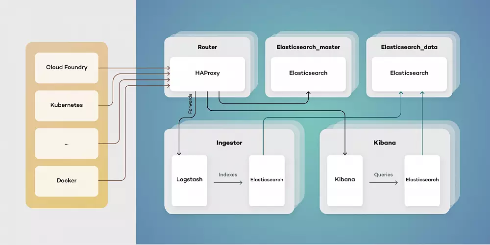
Our proposed architecture consists of five types of virtual machines - Routers, elastic masters, elastic data, ingestors, and Kibana instances. This toolset simplifies scaling of components while separating their responsibilities. Each of them has a different function:

•  Elasticsearch_master - controls indexes and Elasticsearch master. Responsible for creating new indexes, rolling updates and monitoring clusters health.
•  Elasticsearch_data - stores data and retrieves it as needed. Can be run both as hot and warm storage, as well as provides redundancy on data.
•  Ingestor - exposes input endpoints for events both while transforming and enriching data stored in Elasticsearch.
•  Kibana - provides users with visualizations by querying Elasticsearch data.
•  Router - serves as a single point of entry, both for users and services producing data events.

Architecting your Elastic Stack deployment in this way allows for the simple upgrade procedure. Thanks to using a single point of entry, switching to a new version of Elastic Stack is as simple as pointing HAProxy to an upgraded cluster.

Using a clustered structure also allows for freely adding data nodes as needed when your traffic inevitably grows.

This year’s KubeCon was a great occasion to sum up 5 years of Kubernetes and outline its future. It was also a great place to make some important announcements, and we got it. Our team spent those days not only on learning about new features and networking with this amazing community but also talking about how Cloudboostr can impact the adoption of cloud-native technology .

Grape Up team joined 7,700 attendees, top enterprises, media and analysts in Barcelona, Spain at KubeCon + CloudNativeCon Europe 2019 to discuss what’s new in Kubernetes, open source and cloud-native, learn from the most inspiring people in the industry, network with peers from different projects and together work on developing the community gathered around the Cloud Native Computing Foundation.

KubeCon + CloudNativeCon Europe 2019: Kubernetes is thriving

This year’s KubeCon provided us with many promising news and announcements. From the very first keynote to the last workshop, a strong focus was on leading technologies, mainly Kubernetes, and its improvements. Dan Kohn, Executive Director at CNCF, in his opening keynote, presented the Kubernetes place in the cloud-native environment and explained why Kubernetes, like many technologies and applications before, is winning the race called simultaneous invention.

Dan Kohn used engaging storytelling, to present that from ages people have been working on similar ideas at the same time, taking advantage of works done before them. He stressed the fact that there wouldn’t be Kubernetes without technologies, that had built the foundations. He gave us a glimpse of what, in his opinion, makes Kubernetes standing from the crowd:

• It works really well!
• Vendor-Neutral Open Source and Certified Partners.
• The People that develop and promote it.

The end of the opening keynote was strong – all the members of the community gathered around Kubernetes and CNCF have an impact on the technology improvements, as Kubernetes is a foundation on which many new technologies arise.

Hot news: Service Mesh Interface

Microsoft stole the show announcing the launch of Service Mesh Interface, an open project that defines a set of common APIs that provide developers with interoperability across different service mesh technologies.

The Service Mesh Interface includes:

• A standard interface for meshes on Kubernetes.
• A basic feature set for the most common mesh use cases.
• Flexibility to support new mesh capabilities over time.
• Space for the ecosystem to innovate with mesh technology.

This announcement from Microsoft led to many discussions during the conference. As the service mesh is a technology at the early stage of its development, an environment designed for growth should impact its further evolution. SMI is supposed to provide interoperability that will help the emerging ecosystem of tools integrate with existing mesh providers, and instead of doing it individually, gain cross-mesh capabilities through SMI. We’re looking forward to seeing how it will affect the developers' job and help to solve customer problems in the nearest future.

Cloudboostr – an enterprise-grade Kubernetes

What makes KubeCon + CloudNativeCon a special event is an incredible capability of CNCF to engage so many people representing multiple tech and business areas to collaborate together on developing a brighter future for the cloud-native ecosystem. As Dan Kohn said at the beginning of the conference, Kubernetes and parts of the cloud-native landscape build the foundation for the technologies of the future. We at Grape Up also want to participate in this process of developing cloud-native technology and helping various companies implementing Kubernetes.

This is why KubeCon + CloudNativeCon was a great occasion to talk with the end users and developers about their adoption of cloud-native tools. They had a chance to learn more about Cloudboostr, our cloud-native software stack, built with Kubernetes at its core , and allowing companies to stand up a complete cloud-native environment in a couple of hours. Our experts spent those days in Barcelona on discussing the evolution of Kubernetes, its business use cases, and ways to get the most of its capabilities. Our team value this kind of events the most – it's crucial for our product development and a better understanding of people’s challenges and business needs.

Seeing companies highly interested in Cloudboostr capabilities, we are encouraged to work even harder on new improvements. And this the clue to the Kubernetes success – by building a community that inspires other members to grow and connecting them to accelerate the development of associated services, CNCF has created a self-engaging mechanism that helps Kubernetes thrive and acquire new users. This strategy makes Kubernetes an important part of the technology development as a whole, which with every year becomes even more impressive.

Adapting the latest technologies obligates executives to decide if they should build an in-house team or outsource demanding processes and hire an external team. And while outsourced projects become more sophisticated, leaders responsible for making decisions are taking into account more factors than just cost savings. Here comes nearshoring.

Disruptive economy, the fast-changing landscape of cutting-edge technologies, and extremely demanding customers – regardless of the established position on the market, today’s most powerful enterprises need help to retain once gained a competitive advantage . Most of the world’s largest companies are undergoing radical changes that focus on adapting the latest technology and game-changing approaches to company culture.

To embrace digital transformation and get the most out of it, leaders in their fields – automotive, telco, insurance, banking, etc. – utilize knowledge and experience of external teams. As this collaboration is getting more recognition it also takes more sophisticated forms. For decades, the biggest enterprises have been opening their branches in different countries or delegating parts of their processes to specialized teams outside the organization – this is the way outsourcing and offshoring were born.

And while it works perfectly for many business fields, companies that implement the most comprehensive technologies, rebuilding their core businesses, and trying to adopt promising approaches to software delivery, need a solution that is more sophisticated.

What is nearshoring?

Delegating tasks to external teams is full of benefits, but also has some real treats – like cultural differences in communication between teams, challenges to manage processes remotely, disruption in transforming knowledge, and many more. After years of testing good and bad experiences, some enterprises have mastered the most effective way to delegate job – nearshoring.

Nearshoring is often described as the outsourcing of services, especially regarding the newest technologies, to companies in nearby countries. In practice, it means that an enterprise from Germany hires a company from Poland to develop a particular project like building an app or implementing software. Nearshoring is often used by brands expanding their services to the new yet advanced business fields, where building and an in-house team responsible for a given area would be too expensive and challenging.

Why do enterprises prefer nearshoring over offshoring?

While using nearshoring and offshoring comes to some common profits – cost savings, tax benefits, finding skilled professionals in given niches, the first one supposed to be an answer to the challenges addressed in a previous part. Companies that complain about their experiences with offshoring too often make the same mistakes. They decide on moving their processes to the far-distant countries regardless of cultural differences and working style. They focus on thing easier to measure, like financial results and don’t take into consideration less obvious factors.

Backed with that experiences, enterprises from various industries have started to collaborate with teams of professionals that have more in common with their employees; geographically, by living in the same part of the world, often sharing a border, and culturally – by belonging to similar cultural circle, sharing common working culture, and being at a comparable level of language used in project (English, first!).

According to many leaders responsible for workforce management, when deciding on hiring a company that have to help you with improving your business, especially if you're trying to implement complex technology, you should pay at least as much attention to the communication and soft skills as to the know-how and experiences in working on similar projects.

Where do enterprises from Western and Northern Europe look for partners?

Agile teams from Central Europe that consist of experts in transforming businesses, implementing DevOps culture, and enabling cloud-native technologies are getting a strong recognition among established companies from Germany, France, UK. Norway and Italy. Professionals in Poland, Czechia or Hungary are known for their skills, language proficiency, and working culture. And it has never been more difficult to find some real differences in the ways people from these parts of Europe live.

All these things make collaboration more fluent and easier to manage. Partnering with companies from the same time zones can also save the cost of communication and transport, and makes them available during similar working hours.

Taking into account flexibility, language skills, technical knowledge, experience in various international projects, lower operational costs and cultural similarities to the leading European countries, companies from countries like Poland have become natural nearshoring hubs.

Collaboration with top enterprises from a nearshoring partner’s perspective

For the last couple of years, Grape Up has been working as a nearshoring partner with the most recognized brands in various industries like leading automakers from Germany and large telcos from Italy and Switzerland. These experiences have helped our team develop soft skills needed to get the most out of the cooperation, both for hiring enterprises and our employees who can now master their expertise working on demanding projects for the most competitive businesses.

We have to admit that our competitive advantage may seem unfair. We’ve gathered a huge team of experienced engineers familiar with the latest cloud-native technologies, Open Source tools, DevOps and Agile approaches. They feel well in the international environment, speak fluent English, and are good in adapting to a new working style. We have two R&D centers in Poland and a few offices in Europe. We use experience amassed through the years of working with companies that are willing to be early adopters of cutting-edge technologies and innovative methodologies. We’re active contributors to cloud-native and open source communities, we attend top conferences and industry events – that give us direct access to knowledge and innovative ideas. Being ahead of the competitive crowd allows us to focus on the most promising projects.

If your enterprise is working on digital transformation, trying to implement DevOps or adapt cloud-native technologies and you need some support or consultancy reach us without a doubt . We are responsible for numerous successful migration to the cloud, enabling cloud platforms, transforming legacy software into cutting-edge applications, and tackling business challenges that at first sight might seem unsolvable.

Pair programming has become a popular way of developing the newest products and encouraging team members to share knowledge and grow together. Many of the world’s top enterprises adopt this innovative technique. Some of them with success and some of them with less expected results.

Before a company embraces pair programming its leaders and developers should get to know some basic knowledge about this approach. As a company that not only uses this practice on a daily basis but also implements pair programming in the customer’s engineering teams, we’ve answered to the commonly asked questions about this technique, its pros, and cons, how to prepare a workstation for developers working in pairs, and if pair programming is good for everyone.

What is pair programming and how should it look like?

You can find various definitions, but most of them agree that pair programming is an agile software development technique that requires two developers working together on the same block of code, using one workstation. In these pairs, one programmer is becoming a “Driver” and the second one is known as a “Navigator”. Where they work together “Driver” manages a computer and writes code, whereas “Navigator” is supposed to check the written code, follow colleague’s job, and work on problems faced during implementation. When using the pair programming technique, programmers should discuss ongoing works, search for effective solutions, and support each other. What’s important, roles in a pair coding team should be changed during a workday as they are not assigned permanently.

How to prepare a workstation?

The most important thing when designing a workstation comes to making it comfortable for both programmers. A desk for a pair should be properly larger than a desk for an employee working alone. And when two people work together for eight hours a day both need their own, dedicated space to build a comfort zone. A workstation for coding duo requires at least two monitors that displaying the same things, and a keyboard and mouse for each developer.

Teams that work remotely proved that pair programming can be done effectively even when collaborating developers do it at a distance. It’s important to equip these developers with a working gear that enables productive communication, and high-quality headphones are a must-have.

Here is a list of useful tools and resources for pair programming:

• Cloud IDEs: AWS Cloud9, Codenvy,
• Communication and screen sharing tools: Skype, Slack, Zoom, TeamViewer, Stride,
• Live Code Share Extensions: Atom Teletype/VSCode Live Share,
• GIT Scripts: pivotal-legacy/git_scripts.

Advantages and disadvantages of pair programming

And when pair programming delivers real value for companies that implemented this technique, the leaders responsible for adopting these practices in their teams have to be aware of its threats. Here are some of the most valuable pros of pair programming:

• Higher quality of designed solutions - more compound and more meaningful development for given tasks.
• Different views and perspectives regarding the same problem.
• Reduced risk of failure or making a mistake.
• Time and cost savings - software is delivered faster which decreases the costs of development.
• Agile and productive knowledge transfer in projects.
• Breaking down silos in projects - avoiding situations when only one person in a project owns key knowledge.
• Building stronger relationships among team members.

And here come some cons every company has to take into account:

• Dealing with distractions to individual comfort zones and independent working style.
• Personalized working environment - getting used to a non-standard way of doing a job.
• Common lack of convenience to not that obvious and innovative way of programming among developers used to works on their own.
• More demanding and exhausting way of work.

All of the disadvantages may result in rising discomfort and drops in productivity which sabotage the whole idea of pair programming and potential wins it could provide.

Was every developer born for pair programming?

Pair programming may not be that easy as it is often presented. This technique obligates developers to be communicative, conscientious and focused on the subject matter. For many coding professionals, the hardest part of programming in pairs comes to the necessity to adjust to the other person - her/his way of work, time, and individual habits.

People who value working on their own manner and their own comfort, need focus and quiet environment, or just avoiding too much engagement in communication, may find pair programming too demanding for them.

My experiences with PP

My experience with pair programming has started two years ago. The theory seemed reasonable, but I was a little bit skeptical, and to be honest, I didn't believe in promised advantages. For me, it was rather a waste of time and resources when two developers work on the same problem at the same time.

At first, it was hard. I had to change my entire working routine and adjust to a colleague I was paired with. Actually, we both had to modify our working style, and we all know how difficult it is to change habits.

Adjusting to the new technique of doing my job influenced my time after work. I was more tired but at the same time, I felt that we had done a lot of good quality jobs. And step by step, it became easier as we got familiar with those practices. What was really encouraging - the result of our work and the amount of new knowledge was insane .

Working at that level of focus is demanding and costs a lot of energy. So, having a break for 2 or 3 minutes, do some small talk about topics unrelated to problems you’re currently trying to solve, may result in a more productive attitude during the day. It’s also worth noting, that direct collaboration with one of my colleague gave me the opportunity to better get to know that person and having a good friend at work also improved my comfort.

After a few weeks, I’ve noticed all these advantages of pair programming that previously wasn’t that obvious to me. We’ve improved the quality of our work, and our solutions were well thought out. As a result, we’ve minimized the number of mistakes which significantly enriched our outcome. And then it has become clear for me that pair programming is not just a cool theory but an effective way of developing new solutions and useful tool for learning new things. And when it’s a challenging technique, maybe not for everyone, but for sure it’s worth giving it a try. Anyone can try it on his/her own and in case of any troubles get back to the previous way of doing the job.

To sum up all my experiences with pair programming, I have to admit that this technique definitely works and expect the simple tasks, it’s worth to use it every day.

Keeping up with the newest technologies is demanding. A lot of companies tend to do that once in a while, and it is totally understandable. It is hard to follow and discover the perfect momentum to choose the cloud technology that will be valuable and cost-effective for years to come.

Cloud is not only a technology, but it also determines how to design, build and maintain applications and systems. For someone who is currently engaged in the process of digital transformation that is a huge deal – it's like upgrading your rickshaw to the newest Mustang car. All of the development tasks seems to be so easy after adopting to all cloud and DevOps conditions.

The common mistake in the situation where your process and software tools are outdated is to reinvent the new environment by yourself. Especially, when sophisticated platforms or infrastructures come into the picture. Becoming an expert in cloud technologies is a perfect example. It requires a lot of time and resources to master the best tools and to make them work together in the way we want them to. That time should be spent instead on what drives the company’s business and what the customer cares about the most: developing the product that will be running in the cloud.

At Grape Up, we follow a technology agnostic approach. We choose tools and technologies that are tailored to every specific customer and project. While working with the various companies on digital transformation, we helped several teams leverage cloud-native technologies and adapt a DevOps approach to deliver software faster, better, and safer. And despite the fact that every case was different, we have identified a visible pattern. Our team discovered a strong market demand on a cloud-native platform based on open source solutions. We also noticed that in most cases platform maintenance operations were outsourced. Again, building know-how is a hard process, so why not let someone with the right experience lead the way?

This is how Cloudboostr was born. A complete solution to run any workload in any cloud . All based on available open source tools that are well-known by the community and most importantly widely used and maintained. In the beginning, we’ve created a type of reference architecture to accelerate the digital transformation process. It was used as our internal boilerplate, not to reinvent to the whole thing with every customer, but rather use something based on the experiences from previous projects. Along the way, what used to be our template, got mature, and the time has come to make it an external platform, available for other companies.

How does the Cloudboostr platform work?

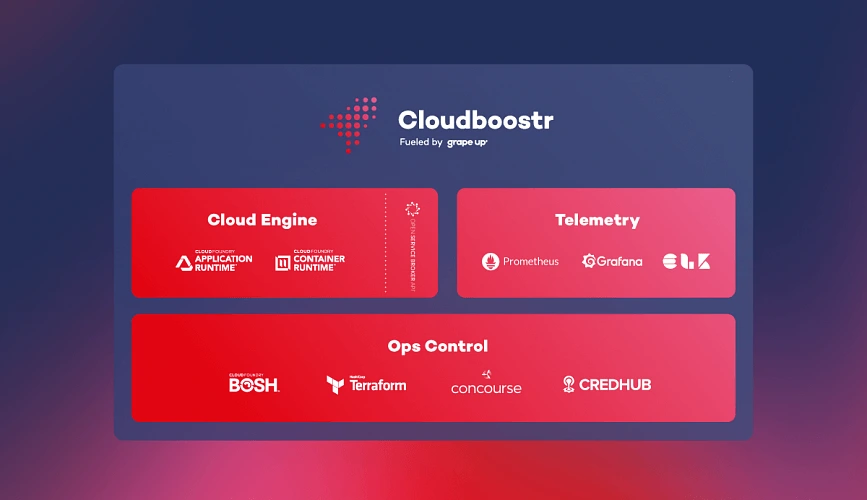
The Cloudboostr’s technology stack incorporates a number of leading open source technologies proven to work well together. Cloudboostr’s Cloud Engine is built with Kubernetes and Cloud Foundry, making applications deployment easy and both solutions cover a wide spectrum of application use cases. Terraform, BOSH & Concourse are used to automate the platform’s management and operations, and also track who, when & why applied a particular change. Built-in Telemetry toolkit consisting of Prometheus, Grafana and ELK stack allows to monitor the whole platform, investigate any issues and also recognize areas which should be improved.

The main abstraction layer of the platform is called Ops Control. It is a control panel for the whole platform. Here, all of the environments and also all shared resources like managing, monitoring or alerting services, are created and configured. Every environment can be created with either Cloud Foundry or Kubernetes or both of them. Shared resources help to monitor and maintain all of the environments and ensure proper workflows. From the operator’s perspective, the main point of interaction is Concourse with all of the pipelines and CLI for more advanced commands. Plus all of the Telemetry dashboards, with all sorts of graphical charts and metrics, where all concerns are clearly visible.

Cloudboostr as a platform includes all of the third party components under its wings. This means that any new platform releases will incorporate not only internal features or improvements but also upgrades of its elements if available. From a perspective of platform user, this is convenient - there is no need to worry about any upgrades, but one - the platform.

From a production perspective, it is crucial to have your platform always up and running. Cloudboostr uses HA-mode by default and leverages the cloud’s multi-AZ capabilities. It also automatically backs up and restores individual components of the platform and their state and data, allowing you to easily recreate and restore a corrupted or failed environment.

It is also important that Cloudboostr comes pre-configured, so if you're starting a journey with the cloud, you can install the platform very fast and be ready to deploy your applications very quickly. The initial cost of getting platform working is fairly low when it comes to getting the know-how, and that's a huge benefit.

How can Cloudboostr be tested?

It is obvious that platform is a big deal and no one would like to buy a pig in a poke. Especially when long term services are in the picture. Grape Up enables customers to try out the platform for a while before making a final decision. It is also understandable that most of the companies need more time to get to know the technology behind the platform. That's why the trial time is done in the dojo style. For a few weeks, the Grape Up crew settles in a customer location, installs the out of the box product, teaches how to use it and also navigates migration of the first application to the platform. Support provided by experienced platform engineers helps to understand the full capabilities of the product and how to use it in particular scenarios.

After the first period, there is another time frame for unassisted tests, where the client’s operations team can play with the platform, apply various tests or migrate other applications to see how they will run on the new environment. During that time, Grape Up platform engineers are still available to help and guide.

What about costs?

All the mentioned technologies are open source and if one would like to build this platform on their own they can do that. So why should anyone pay for that? The answer is, no one needs to pay for Cloudboostr license – it's totally free.

In order to use Cloudboostr platform though, you need to have a support service subscription plan. It's obvious that complex solutions, such as cloud platforms, need to be maintained by someone. Majority of the market outsource the services, which is especially convenient if you use software organized as a product. Again, it's not worth it to gain experience by yourself and spend weeks or months on that, while your competitors are moving forward. Also knowing that there is already a fair share of the market, who knows the technical details that you're looking for. However if one feels that they already have all of the knowledge needed to maintain the platform themselves, that's fine too - they can simply choose a minimal support plan.

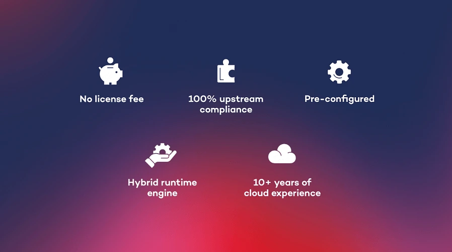
Conclusion

The wisdom coming out from this article is – if you want to go cloud, do not reinvent the cloud wheel from scratch. Do the things that you were meant to – focus on building your applications and delivering true value to your customers and let the experts help you run your applications in the cloud and maintain the cloud environment. Boost your cloud journey with Cloudboostr !

Cloud Foundry Summit 2019 in Philadelphia was the first event on our list of conferences we're heading to this year. It was an excellent season opening and another example that Cloud Foundry community is developing well. "Building the future" - this year’s motto is a good metaphor for the current situation. Cloud Foundry is evolving, and it's perfectly fine.

A quote from Abby Kearns, Executive Director of the Cloud Foundry Foundation, can summarize what's happening these days:

“We’re all kayakers now, navigating the rapids of change. The quickest learners will be the biggest winners.”

Abby Kearns started the summit with this powerful statement, and she addressed the fact that influence the way we develop our companies – technology is evolving at a rapid pace. The cloud-native landscape is continuously growing as new solutions and ideas are introduced on a regular basis. Often easy to use, but not developed enough to use them on production without taking some risk. How to choose the right technologies? When to adopt them? Should the whole application or component be rewritten? As Abby said, the quickest learners will be the biggest winners.

During the event, we had a chance to see how many of those tools have evolved into more mature and more customer-friendly apps. From the end-user perspective, it was promising to see them working together, as it gives a glimpse of how it may look in the future.

Cloud Foundry loves Kubernetes

One of the hottest topics in the corridors was for sure the Eirini project. This is a perfect example of how software should evolve – and yes, Cloud Foundry Foundation isn’t too proud to admit that Kubernetes is better than Diego/Garden in particular cases. This is how one open source should work with another.

A year ago one could ask if Kubernetes will push Cloud Foundry into the shadow. The question was wrong – how could we compare apples and oranges? To simplify things, we can call Cloud Foundry an Application PaaS, while Kubernetes can be described as a Container PaaS. This year we’re discussing how they can work together. As this seems to be the right question the Eirini project may be the right answer.

We can't wait to hear more about Cloud Foundry and Kubernetes collaboration. Especially given the fact that the project was proclaimed to pass core functional tests and it is ready early adopters.  Learn more about Project Eirini

Interoperability

One of the keywords announcing the conference was interoperability. Eirini is a good example of that. TheCloud Foundry project continues to integrate with other open source projects to provide more capabilities for users. Platform maturity allows to incorporate new tools easily and makes the whole process user-friendly.

Worth noting is the fact that all of these tools are somehow used (or will be used soon) in ongoing projects, so it's not just state of the art. This is for sure a hard work of the community experts that help Cloud Foundry stay ahead of the curve.

The Comcast story

Philadelphia is home to a large Cloud Foundry member – Comcast. The company story of successful digital transformation is a practical guideline on how it should look like. In this year's agenda there was no case study about it, but anyway it is worth mentioning and congratulating the Comcast crew. This technology voyage and company restructuring – to be explicit, breaking siloses – should be an inspiration to all of us.

Cloudboostr

It wouldn't be an honest review without writing some personal summary of how do we feel about our participation in the summit. As an IT consulting company, we were more than excited to be a Silver Sponsor of a conference which gathers hundreds, if not thousands of cloud experts in one place.

Besides an engaging business case study of helping an established company to go through a digital transformation, we've also seen a huge interest in  our cloud platform - Cloudboostr . A lot of companies want to automate their deployment & delivery tools. Becoming a cloud expert is a long and demanding process for firms that need to be focused on running their business operations. Majority of the world's top enterprises collaborate with external teams. Some of them use proven solutions that help them adjust to the fast-changing environment. A complete cloud platform (not only PaaS) meets market needs perfectly, and we were happy to tell our new friends about it.

As the "kayakers" we know that it's a long way to go and we'll be happy to share our knowledge and experience in order to help our customers move forward.

Working as a platform operator with cloud-native technologies, L2 technical support , and participating in CF installations give a unique opportunity to observe how different companies implement new technologies in their works and how they deal with running large production environments. Among various bad experiences, imperfect ideas, and the most reprehensible habits related to running and maintaining cloud infrastructures those listed below can generate the most complicated problems.

Bad practices often occur when it comes to productive CF infrastructures. However, these guidelines should help everyone who runs or uses any of the production-ready workloads.

Neglected capacity planning

Let’s start with this: you have to be aware that you will run out of resources eventually. Then you should plan how to scale up. If you run on-premises software, you should consider hardware and virtualization layer’s requirements. Proper sizing of the availability zones will always save you many problems.

On top of IaaS there is always a PaaS or some container orchestrator. The key to success here is to optimize all the limits, quotas and other configurations (like application scaling rules, etc.) so the microservices never consume available resources, even under high load.

It’s obvious that both hardware and virtualized capacity planning requires a buffer. You need to be prepared for issues, maintenance and infrastructure changes. There is no best configuration. It always depends on many factors but nevertheless, it is always worth taking into consideration.

Capacity and resources have to be monitored. A good monitoring tool with decent alerting rules will help you predict possible problems and react quickly if anything bad happens to your infrastructure.

Poor or no CI/CD

If you want to maintain any piece of software, don’t forget how valuable is automation. Many times people quit on CI/CD implementation because of the deadline or tasks formally more important. In most cases, it doesn't end up well.

It's hard to build, test and deploy software without automation. The manual process is highly exposed to the risk of human error. Apart from that, it is almost impossible to keep track of deployed software (version, updates, hotfixes, security patches, etc.) in large production environments. Sometimes you have to maintain CF platforms hosting 1K+ applications. Consider how problematic would be the migration process if there is a business decision to switch to a different solution.

For operators maintaining the infrastructures, platforms, and services used by developers it’s critical to keep everything up to date, take care of security patches and configuration changes. It is impossible to handle this manually with minimal or zero downtime of the services. That is why automated pipelines are so important, and you should never give up on implementing them in the first place.

Poor or no backup/restore procedures

Backup/restore is another important process that people often put in the background. You may think that your applications are safe if your IaaS offers you a highly available environment or containers you run have an auto-healing function. This is not true. Any disaster can happen, and in order to recover quickly, you have to create a well-defined backup and restore procedures that work. That’s not all, as the procedures have to be tested periodically. You need to be sure that backup/restore works fine since the process may depend on some external services that might have changed or just brake.

No periodic updates

Every software has to be updated regularly in order to keep it secure. It is also much safer to perform minor updates with a little chance of failure or downtime than doing ‘big jumps’. Major updates introduce higher risk, and it is hard to catch up with versions especially if there is no automation implemented.

You may see cloud infrastructures that were just installed and never upgraded and that generates a lot of issues for platform operators (users can’t see any difference). It is not a problem until everything works correctly. But after some time people may start escalating issues related to the versioning of the services. Unfortunately, it is too late to upgrade smoothly. It becomes a big spider’s web of dependencies. It may take weeks to plan the upgrade process and months to execute it.

Flawed architecture

Defective architecture generates serious problems. Many times developers are not aware of the issue until it shows up in production. After that, it’s really hard to admit the architecture needs to be changed and people often try to get rid of the effect instead of fixing the cause of the problem.

Let’s take a real-life example often faced. You may be receiving Prometheus alerts saying that ELK stack is overloaded. After investigating the issue, it may turn out that microservices are so verbose that they generate thousands of log messages per second. What if you raise the possible architecture problem, but nobody cares? As a result, you’ll have to scale ELK. In those cases, it may waste hundreds of CPUs and terabytes of memory and storage. That makes somebody spend money just to store 90% of useless data and maybe 10% of valuable information. This is really a simple way to put yourself in a situation without a way out.

Conclusion

Following these guidelines will definitely not be easy. Sometimes people responsible for making decisions are just not aware of the consequences of taking some actions. The role of every technically skilled person in the project is to spread the knowledge and make people aware of what may happen if they ignore those basic rules that matter. You can’t step back if you encounter such practices in the future. Be an example for others and drive change - it’s always worth trying.

In one of his latest articles, Filip Ryba describes the  specificity of working on on-site projects in the USA . Let's compare his experiences with similar projects run in other parts of the world.

Let's take the US first.

What can we learn from U.S work culture?

Teams in the USA are very customer-oriented and everyone knows their users. Ask your teammate about some functionality in the product. In Poland you will usually get a technical answer, something along the lines "Oh, it is because we need to get additional data from..." and you have to ask some follow-up questions, to get to actual functionality needed by customers and in many cases, you won't get that answer at all. In the USA you will most likely get "Oh, it is because our customers need to know if...", which puts you in the right business context from the start. I find it really positive since instead of just focusing on technical parts you are focusing more on the actual usability of the feature for the customers.

The teams that I worked with always had a flat structure. Sure, there was a PM and a PO, but they were sitting with their team at the same desks. It's another factor that makes communication super easy and effective.

We are actually closer culturally to the United States than you might think. We have Hollywood movies in our cinemas and on TV, we listen to news involving the US, and Netflix becomes popular worldwide. It gives us something to talk about to break the ice.

Obviously, everyone there speaks English, although its level differs from person to person. It is pretty common especially in IT that teams are multi-cultured and you will have teammates from India, China, Mexico to name a few. This might be challenging at first, but you will catch up pretty quick. Being constantly exposed to a foreign language is the best way to learn.

Another aspect of American culture that is especially contrasting with our culture is that when you share something you will always get positive feedback. You will hear "Oh, that's great!" or "Oh, that's so cool!" and it does not matter if they really think that. What matters is that it encourages to share more and it works.

Differences between American and German working culture

How do they compare to our neighbors from Germany? While the teams here also have a flat structure there is also a more rigorous division of responsibilities between teams. There are parts that belong to the architecture team, testing team, CI/CD teams, etc. This inevitably leads to more internal dependencies and generates more meetings. The Germans are very polite and open to discuss everything. Even if they do not have to agree with you, they will at least hear you out. Even when a decision comes from the top, they will still seek consensus within a team.

While collaborating with German companies your PO/PM will be more technical than their US counterpart. Firstly, it helps to translate business goals to engineering tasks. Secondly, the goals that do not bring immediate business value like code refactoring or improvements to the development environment are better understood, and easier accepted. All of that makes projects more technical with teams having less influence on the business side of the product.

Collaborating with Italian teams

The US might be 7000 km from Poland, but we are culturally closer to them than let’s say Italy. If you add to it that not many Italians speak English, the communication may be a bit challenging. The project I worked on was managed in a more freestyle manner. When seeking some information about a project all you have to do is to walk around the office and ask around until you find someone who has that knowledge. Of course, sometimes you also have to find someone who can help you as a translator.

Due to the same reasons communication with an end user is next to impossible. Trying to change the way things are done is even more challenging. Let’s say you finally encouraged your PM to agree to change things a bit. You go back home happy that things are finally moving into the right direction only to discover next day that there was another meeting with some other PM’s and everything is going back to how it was. Sometimes it requires time to work out a way of running projects that suits both sides - when you deal with the early struggles the job becomes more effective.

Collaborating with people from other countries sometimes may be demanding but when you invest some time in better understanding their work culture, a way of communicating, and daily routines it becomes easier. Despite all the differences and challenges at the beginning, on-site projects can be a valuable lesson and helpful experience. There is one more aspect of working abroad that I really like. You can of course visit the same countries by yourself during vacation. However as a tourist you don’t have to figure out what is the best way to commute, where to go shopping, where to eat, what to do on Friday evening etc. This allows you to experience how it is to live there without actually moving there.

Cloud is everywhere these days. There is no doubt about that. Everyone already did or is about to make an important decision - which cloud provider to choose?

For enterprise solutions, the first thought goes to the big players: Amazon, Microsoft, Google. They provide both private and public cloud solutions using their own set of APIs, command-line tools and of course pricing.

It is very easy to get in, but is it the same with getting out? All your services may already benefit from great tools and services shared by your provider. Awesome tools, but specific to the company. Does Amazon CLI work with Azure? Not really.

The important part is that the scale of your infrastructure you can manage. The software can be optimized, to some point, but still, it may be a viable choice. Resources can be hosted using CDN to better manage bandwidth and storage cost. But what can be done if the provider increased the prices? How this can be mitigated?

The exit strategy

This is why you need an exit strategy. The plan to move all your resources safely and possibly without any interruptions from one warehouse to another. Or even the plan to migrate from one provider to the another. The reasons for the change may be very different. Pricing change, network problems, low latency or even a law change. All this may push your company against the wall. It is fine when you are prepared, but how to do this?

It may seem more on the paranoic side or catastrophic thinking, but in reality, it is not so uncommon. Even worse case, which is a provider shut down, happened a lot lately. It is especially visible with an example of cloud storage startups. $15 million dollars CloudMine startup filed for bankruptcy last year. A few years ago the same thing happened to Nirvanix and Megacloud. Nobody expected that and a lot of companies has been facing that problem - how can we safely move all the data if everything can disappear in 2 weeks?

Does it mean AWS will go down tomorrow? Probably not, but would you like to bet if it will be there in 10 years? A few years ago nobody even heard about Alibaba Cloud, and now they have 19 datacenters worldwide. The world is moving so fast that nobody can say what tomorrow brings.

How to mitigate the problem?

So we have established what the problem is. Now let’s move to the solutions. In the following paragraphs, I will briefly paint a picture of what consists of an exit strategy and may help you move towards it.

One of them is to use a platform like Cloud Foundry or Kubernets which can enable you to run your services on any cloud. All big names offer some kind of hosted Kubernetes solutions: Amazon ECS, Microsoft AKS and Google GKE. Moving workloads from one Kubernetes deployment to another, even private hosted, is easy.

This may not be enough though. Sometimes you have more than containers deployed. The crucial part then will be to have infrastructure as a config. Consider if the way you deploy your platform to IaaS is really transferable? Do you use provider-specific databases, storage or services? Maybe you should change some solutions to more universal ones?

Next part will be to make sure services your write, deploy and configure are truly cloud-native. Are they really portable in a way you can get the same source code or docker image and run on the different infrastructure? Are all external services loosely coupled and bounded to your application so you can easily exchange them? Or if all your microservices platforms are independent?

Last, but not least is to backup everything. Really, EVERYTHING. Not just all your data, but also the configuration of services, infrastructure, and platforms. If you can restore everything from the ground up to the working platform in 24 hours you are better than most of your competitors.

So why do I need one?

Avoiding provider lock-in may not be easy, especially when your company just started to use AWS or Azure. You may not feel very comfortable creating an exit strategy for different providers or just don’t know where to start. There are solutions, like Grape Up’s Cloudboostr, that manage backups and multi-cloud interoperability out of the box. Using this kind of platform may save you a lot of pain.

An exit strategy gives you a lot of freedom. New, small cloud provider comes to the market and gives you a very competitive price? You can move all your services to their infrastructure. Especially when we consider that small cloud providers can be more flexible and more keen to adapt to their client needs.

An exit plan gives safety, freedom, and security. Do not think of it as optional. The whole world goes toward the multi-cloud and the hybrid cloud . According to Forbes, this is what 2019 will matter most in the cloud ecosystem. Do you want to stay behind? Or are you already prepared for the worse?