Accelerating data projects with parallel computing

Inspired by Petabyte Scale Solutions from CERN
The Large Hadron Collider (LHC) accelerator is the biggest device humankind has ever created. Handling enormous amounts of data it produces has required one of the biggest computational infrastructures on the earth. However, it is quite easy to overwhelm even the best supercomputer with inefficient algorithms that do not correctly utilize the full power of underlying, highly parallel hardware. In this article, I want to share insights born from my meeting with the CERN people, particularly how to validate and improve parallel computing in the data-driven world.
Struggling with data on the scale of megabytes (10 6 ) to gigabytes (10 9 ) is the bread and butter for data engineers, data scientists, or machine learning engineers. Moving forward, the terabyte (10 12 ) and petabyte (10 15 ) scale is becoming increasingly ordinary, and the chances of dealing with it in everyday data-related tasks keep growing. Although the claim "Moore's law is dead!" is quite a controversial one, the fact is that single-thread performance improvement has slowed down significantly since 2005. This is primarily due to the inability to increase the clock frequency indefinitely. The solution is parallelization - mainly by an increase in the numbers of logical cores available for one processing unit.

Knowing it, the ability to properly parallelize computations is increasingly important.
In a data-driven world, we have a lot of ready-to-use, very good solutions that do most of the parallel stuff on all possible levels for us and expose easy-to-use API. For example, on a large scale, Spark or Metaflow are excellent tools for distributed computing; at the other end, NumPy enables Python users to do very efficient matrix operations on the CPU, something Python is not good at all, by integrating C, C++, and Fortran code with friendly snake_case API. Do you think it is worth learning how it is done behind the scenes if you have packages that do all this for you? I honestly believe this knowledge can only help you use these tools more effectively and will allow you to work much faster and better in an unknown environment.
The LHC lies in a tunnel 27 kilometers (about 16.78 mi) in circumference, 175 meters (about 574.15 ft) under a small city built for that purpose on the France–Switzerland border. It has four main particle detectors that collect enormous amounts of data: ALICE, ATLAS, LHCb, and CMS. The LHCb detector alone collects about 40 TB of raw data every second. Many data points come in the form of images since LHCb takes 41 megapixels resolution photos every 25 ns. Such a huge amount of data must be somehow compressed and filtered before permanent storage. From the initial 40 TB/s, only 10G GB/s are saved on disk – the compression ratio is 1:4000!
It was a surprise for me that about 90% of CPU usage in LHCb is done on simulation. One may wonder why they simulate the detector. One of the reasons is that a particle detector is a complicated machine, and scientists at CERN use, i.e., Monte Carlo methods to understand the detector and the biases. Monte Carlo methods can be suitable for massively parallel computing in physics.

Let us skip all the sophisticated techniques and algorithms used at CERN and focus on such aspects of parallel computing, which are common regardless of the problem being solved. Let us divide the topic into four primary areas:
- SIMD,
- multitasking and multiprocessing,
- GPGPU,
- and distributed computing.
The following sections will cover each of them in detail.
SIMD
The acronym SIMD stands for Single Instruction Multiple Data and is a type of parallel processing in Flynn's taxonomy .
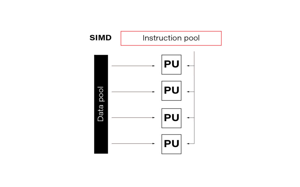
In the data science world, this term is often so-called vectorization. In practice, it means simultaneously performing the same operation on multiple data points (usually represented as a matrix). Modern CPUs and GPGPUs often have dedicated instruction sets for SIMD; examples are SSE and MMX. SIMD vector size has significantly increased over time.
Publishers of the SIMD instruction sets often create language extensions (typically using C/C++) with intrinsic functions or special datatypes that guarantee vector code generation. A step further is abstracting them into a universal interface, e.g., std::experimental::simd from C++ standard library. LLVM's (Low Level Virtual Machine) libcxx implements it (at least partially), allowing languages based on LLVM (e.g., Julia, Rust) to use IR (Intermediate Representation – code language used internally for LLVM's purposes) code for implicit or explicit vectorization. For example, in Julia, you can, if you are determined enough, access LLVM IR using macro @code_llvm and check your code for potential automatic vectorization.
In general, there are two main ways to apply vectorization to the program:
- auto-vectorization handled by compilers,
- and rewriting algorithms and data structures.
For a dev team at CERN, the second option turned out to be better since auto-vectorization did not work as expected for them. One of the CERN software engineers claimed that "vectorization is a killer for the performance." They put a lot of effort into it, and it was worth it. It is worth noting here that in data teams at CERN, Python is the language of choice, while C++ is preferred for any performance-sensitive task.
How to maximize the advantages of SIMD in everyday practice? Difficult to answer; it depends, as always. Generally, the best approach is to be aware of this effect every time you run heavy computation. In modern languages like Julia or best compilers like GCC, in many cases, you can rely on auto-vectorization. In Python, the best bet is the second option, using dedicated libraries like NumPy. Here you can find some examples of how to do it.
Below you can find a simple benchmarking presenting clearly that vectorization is worth attention.
import numpy as np

from timeit import Timer


# Using numpy to create a large array of size 10**6

array = np.random.randint(1000, size=10**6)


# method that adds elements using for loop

def add_forloop():

  new_array = [element + 1 for element in array]


# Method that adds elements using SIMD

def add_vectorized():

  new_array = array + 1


# Computing execution time

computation_time_forloop = Timer(add_forloop).timeit(1)

computation_time_vectorized = Timer(add_vectorized).timeit(1)


# Printing results

print(execution_time_forloop) # gives 0.001202600

print(execution_time_vectorized) # gives 0.000236700
Multitasking and Multiprocessing
Let us start with two confusing yet important terms which are common sources of misunderstanding:
- concurrency: one CPU, many tasks,
- parallelism: many CPUs, one task.
Multitasking is about executing multiple tasks concurrently at the same time on one CPU. A scheduler is a mechanism that decides what the CPU should focus on at each moment, giving the impression that multiple tasks are happening simultaneously. Schedulers can work in two modes:
- preemptive,
- and cooperative.
A preemptive scheduler can halt, run, and resume the execution of a task. This happens without the knowledge or agreement of the task being controlled.
On the other hand, a cooperative scheduler lets the running process decide when the processes voluntarily yield control or when idle or blocked, allowing multiple applications to execute simultaneously.
Switching context in cooperative multitasking can be cheap because parts of the context may remain on the stack and be stored on the higher levels in the memory hierarchy (e.g., L3 cache). Additionally, code can stay close to the CPU for as long as it needs without interruption.
On the other hand, the preemptive model is good when a controlled task behaves poorly and needs to be controlled externally. This may be especially useful when working with external libraries which are out of your control.
Multiprocessing is the use of two or more CPUs within a single Computer system. It is of two types:
- Asymmetric - not all the processes are treated equally; only a master processor runs the tasks of the operating system.
- Symmetric - two or more processes are connected to a single, shared memory and have full access to all input and output devices.
I guess that symmetric multiprocessing is what many people intuitively understand as typical parallelism.
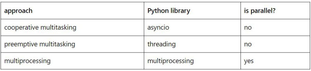
Below are some examples of how to do simple tasks using cooperative multitasking, preemptive multitasking, and multiprocessing in Python. The table below shows which library should be used for each purpose.
- Cooperative multitasking example:
import asyncio

import sys

import time


# Define printing loop

async def print_time():

    while True:

        print(f"hello again [{time.ctime()}]")

        await asyncio.sleep(5)


# Define stdin reader

def echo_input():

    print(input().upper())


# Main function with event loop

async def main():


asyncio.get_event_loop().add_reader(

        sys.stdin,

        echo_input

    )

    await print_time()


# Entry point

asyncio.run(main())
Just type something and admire the uppercase response.
- Preemptive multitasking example:
import threading

import time


# Define printing loop

def print_time():

    while True:

        print(f"hello again [{time.ctime()}]")

        time.sleep(5)


# Define stdin reader

def echo_input():

    while True:

        message = input()

        print(message.upper())


# Spawn threads

threading.Thread(target=print_time).start()

threading.Thread(target=echo_input).start()
The usage is the same as in the example above. However, the program may be less predictable due to the preemptive nature of the scheduler.
- Multiprocessing example:
import time

import sys

from multiprocessing import Process


# Define printing loop

def print_time():

    while True:

        print(f"hello again [{time.ctime()}]")

        time.sleep(5)


# Define stdin reader

def echo_input():

    sys.stdin = open(0)

    while True:

        message = input()

        print(message.upper())


# Spawn processes

Process(target=print_time).start()

Process(target=echo_input).start()
Notice that we must open stdin for the echo_input process because this is an exclusive resource and needs to be locked.
In Python, it may be tempting to use multiprocessing anytime you need accelerated computations. But processes cannot share resources while threads / asyncs can. This is because a process works with many CPUs (with separate contexts) while threads / asyncs are stuck to one CPU. So, you must use synchronization primitives (e.g., mutexes or atomics), which complicates source code. No clear winner here; only trade-offs to consider.
Although that is a complex topic, I will not cover it in detail as it is uncommon for data projects to work with them directly. Usually, external libraries for data manipulation and data modeling encapsulate the appropriate code. However, I believe that being aware of these topics in contemporary software is particularly useful knowledge that can significantly accelerate your code in unconventional situations.
You may find other meanings of the terminology used here. After all, it is not so important what you call it but rather how to choose the right solution for the problem you are solving.
GPGPU
General-purpose computing on graphics processing units (GPGPU) utilizes shaders to perform massive parallel computations in applications traditionally handled by the central processing unit.
In 2006 Nvidia invented Compute Unified Device Architecture (CUDA) which soon dominated the machine learning models acceleration niche. CUDA is a computing platform and offers API that gives you direct access to parallel computation elements of GPU through the execution of computer kernels.
Returning to the LHCb detector, raw data is initially processed directly on CPUs operating on detectors to reduce network load. But the whole event may be processed on GPU if the CPU is busy. So, GPUs appear early in the data processing chain.
GPGPU's importance for data modeling and processing at CERN is still growing. The most popular machine learning models they use are decision trees (boosted or not, sometimes ensembled). Since deep learning models are harder to use, they are less popular at CERN, but their importance is still rising. However, I am quite sure that scientists worldwide who work with CERN's data use the full spectrum of machine learning models.
To accelerate machine learning training and prediction with GPGPU and CUDA, you need to create a computing kernel or leave that task to the libraries' creators and use simple API instead. The choice, as always, depends on what goals you want to achieve.
For a typical machine learning task, you can use any machine learning framework that supports GPU acceleration; examples are TensorFlow, PyTorch, or cuML , whose API mirrors Sklearn's. Before you start accelerating your algorithms, ensure that the latest GPU driver and CUDA driver are installed on your computer and that the framework of choice is installed with an appropriate flag for GPU support. Once the initial setup is done, you may need to run some code snippet that switches computation from CPU (typically default) to GPU. For instance, in the case of PyTorch, it may look like that:
import torch


torch.cuda.is_available()

def get_default_device():

    if torch.cuda.is_available():

        return torch.device('cuda')

    else:

        return torch.device('cpu')

device = get_default_device()

device
Depending on the framework, at this point, you can process as always with your model or not. Some frameworks may require, e. g. explicit transfer of the model to the GPU-specific version. In PyTorch, you can do it with the following code:
net = MobileNetV3()

net = net.cuda()
At this point, we usually should be able to run .fit(), .predict(), .eval(), or something similar. Looks simple, doesn't it?
Writing a computing kernel is much more challenging. However, there is nothing special about computing kernel in this context, just a function that runs on GPU.
Let's switch to Julia; it is a perfect language for learning GPU computing. You can get familiar with why I prefer Julia for some machine learning projects here . Check this article if you need a brief introduction to the Julia programming language.
Data structures used must have an appropriate layout to enable performance boost. Computers love linear structures like vectors and matrices and hate pointers, e. g. in linked lists. So, the very first step to talking to your GPU is to present a data structure that it loves.
using Cuda


# Data structures for CPU

N = 2^20

x = fill(1.0f0, N)  # a vector filled with 1.0

y = fill(2.0f0, N)  # a vector filled with 2.0


# CPU parallel adder

function parallel_add!(y, x)

    Threads.@threads for i in eachindex(y, x)

        @inbounds y[i] += x[i]

    end

    return nothing

end


# Data structures for GPU

x_d = CUDA.fill(1.0f0, N)

# a vector stored on the GPU filled with 1.0

y_d = CUDA.fill(2.0f0, N)

# a vector stored on the GPU filled with 2.0


# GPU parallel adder

function gpu_add!(y, x)

    CUDA.@sync y .+= x

    return

end
GPU code in this example is about 4x faster than the parallel CPU version. Look how simple it is in Julia! To be honest, it is a kernel imitation on a very high level; a more real-life example may look like this:
function gpu_add_kernel!(y, x)

    index = (blockIdx().x - 1) * blockDim().x + threadIdx().x

    stride = gridDim().x * blockDim().x

    for i = index:stride:length(y)

        @inbounds y[i] += x[i]

    end

    return

end
The CUDA analogs of threadid and nthreads are called threadIdx and blockDim. GPUs run a limited number of threads on each streaming multiprocessor (SM). The recent NVIDIA RTX 6000 Ada Generation should have 18,176 CUDA Cores (streaming processors). Imagine how fast it can be even compared to one of the best CPUs for multithreading AMD EPYC 7773X (128 independent threads). By the way, 768MB L3 cache (3D V-Cache Technology) is amazing.
Distributed Computing
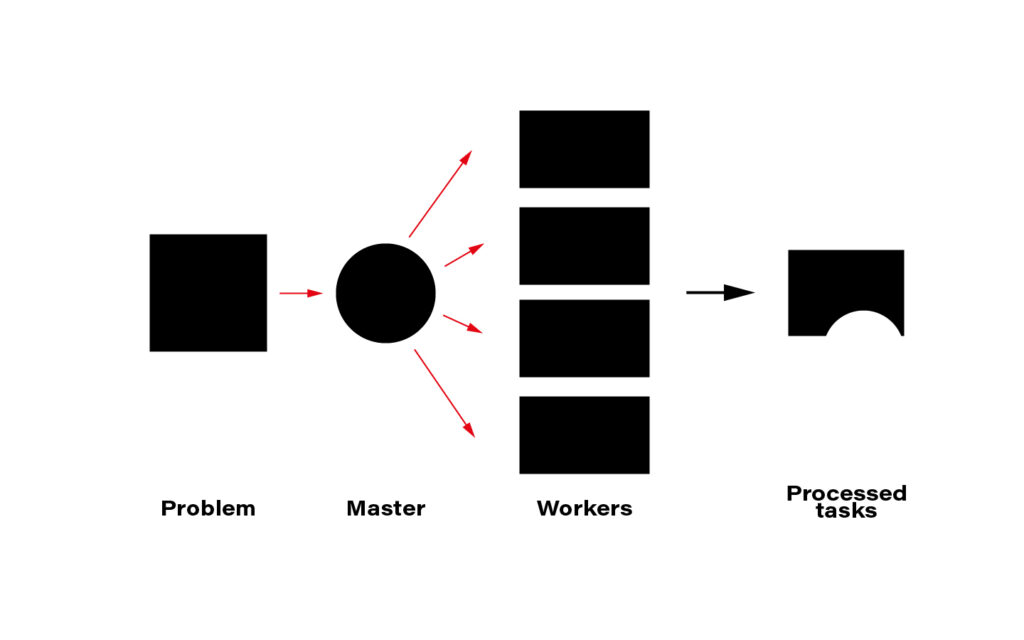
The term distributed computing, in simple words, means the interaction of computers in a network to achieve a common goal. The network elements communicate with each other by passing messages (welcome back cooperative multitasking). Since every node in a network usually is at least a standalone virtual machine, often separate hardware, computing may happen simultaneously. A master node can split the workload into independent pieces, send them to the workers, let them do their job, and concatenate the resulting pieces into the eventual answer.
The computer case is the symbolic border line between the methods presented above and distributed computing. The latter must rely on a network infrastructure to send messages between nodes, which is also a bottleneck. CERN uses thousands of kilometers of optical fiber to create a huge and super-fast network for that purpose. CERN's data center offers about 300,000 physical and hyper-threaded cores in a bare-metal-as-a-service model running on about seventeen thousand servers. A perfect environment for distributed computing.
Moreover, since most data CERN produces is public, LHC experiments are completely international - 1400 scientists, 86 universities, and 18 countries – they all create a computing and storage grid worldwide. That enables scientists and companies to run distributed computing in many ways.

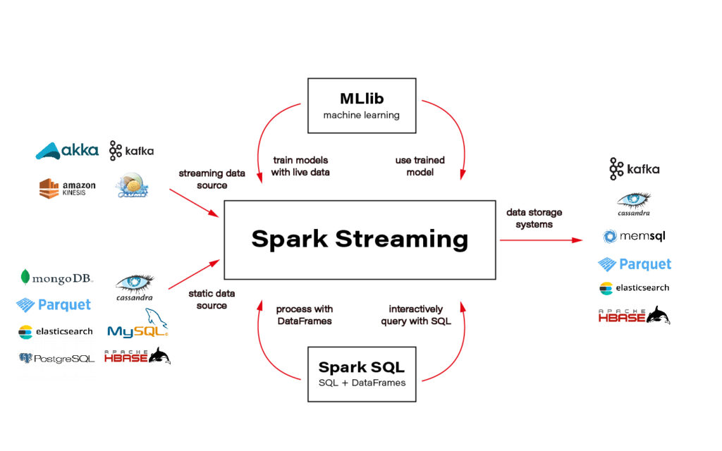
Although this is important, I will not cover technologies and distributed computing methods here. The topic is huge and very well covered on the internet. An excellent framework recommended and used by one of the CERN scientists is Spark + Scala interface. You can solve almost every data-related task using Spark and execute the code in a cluster that distributes computation on nodes for you.
Ok, the only piece of advice: be aware of how much data you send to the cluster - transferring big data can ruin all the profit from distributing the calculations and cost you a lot of money.
Another excellent tool for distributed computation on the cloud is Metaflow. I wrote two articles about Metaflow: introduction and how to run a simple project . I encourage you to read and try it.
Conclusions
CERN researchers have convinced me that wise parallelization is crucial to achieving complex goals in the contemporary Big Data world. I hope I managed to infect you with this belief. Happy coding!

Grape Up guides enterprises on their data-driven transformation journey
Ready to ship? Let's talk.
Check related articles
Read our blog and stay informed about the industry's latest trends and solutions.
How to get effective computing services: AWS Lambda
In the modern world, we are constantly faced with the need not only to develop applications but also to provide and maintain an environment for them. Writing scalable, fault-tolerant, and responsive programs is hard, and on top of that, you’re expected to know exactly how many servers, CPUs, and how much memory your code will need to run – especially when running in the Cloud. Also, developing cloud native applications and microservice architectures make our infrastructure more and more complicated every time.
So, how not worry about underlying infrastructure while deploying applications? How do get easy-to-use and manage computing services? The answer is in serverless applications and AWS Lambda in particular.
What you will find in this article:
- What is Serverless and what we can use that for?
- Introduction to AWS Lambda
- Role of AWS Lambda in Serverless applications
- Coding and managing AWS Lambda function
- Some tips about working with AWS Lambda function
What is serverless?
Serverless computing is a cloud computing execution model in which the cloud provider allocates machine resources on-demand, taking care of the servers on behalf of their customers. Despite the name, it does not involve running code without servers, because code has to be executed somewhere eventually. The name “serverless computing” is used because the business or person that owns the system does not have to purchase, rent, or provision servers or virtual machines for the back-end code to run on. But with provided infrastructure and management you can focus on only writing code that serves your customers.
Software Engineers will not have to take care of operating system (OS) access control, OS patching, provisioning, right-sizing, scaling, and availability. By building your application on a serverless platform, the platform manages these responsibilities for you.
The main advantages of AWS Serverless tools are :
- No server management – You don’t have to provision or maintain any servers. There is no software or runtime to install or maintain.
- Flexible scaling – You can scale your application automatically.
- High availability – Serverless applications have built-in availability and fault tolerance.
- No idle capacity – You don't have to pay for idle capacity.
- Major languages are supported out of the box - AWS Serverless tools can be used to run Java, Node.js, Python, C#, Go, and even PowerShell.
- Out of the box security support
- Easy orchestration - applications can be built and updated quickly.
- Easy monitoring - you can write logs in your application and then import them to Log Management Tool.
Of course, using Serverless may also bring some drawbacks:
- Vendor lock-in - Your application is completely dependent on a third-party provider. You do not have full control of your application. Most likely, you cannot change your platform or provider without making significant changes to your application.
- Serverless (and microservice) architectures introduce additional overhead for function/microservice calls - There are no “local” operations; you cannot assume that two communicating functions are located on the same server.
- Debugging is more difficult - Debugging serverless functions is possible, but it's not a simple task, and it can eat up lots of time and resources.
Despite all the shortcomings, the serverless approach is constantly growing and becoming capable of more and more tasks. AWS takes care of more and more development and distribution of serverless services and applications. For example, AWS now provides not only Lambda functions(computing service), but also API Gateway(Proxy), SNS(messaging service), SQS(queue service), EventBridge(event bus service), and DynamoDB(NoSql database).
Moreover, AWS provides Serverless Framework which makes it easy to build computing applications using AWS Lambda. It scaffolds the project structure and takes care of deploying functions, so you can get started with your Lambda extremely quickly.
Also, AWS provides the specific framework to build complex serverless applications - Serverless Application Model (SAM). It is an abstraction to support and combine different types of AWS tools - Lambda, DynamoDB API Gateway, etc.
The biggest difference is that Serverless is written to deploy AWS Lambda functions to different providers. SAM on the other hand is an abstraction layer specifically for AWS using not only Lambda but also DynamoDB for storage and API Gateway for creating a serverless HTTP endpoint. Another difference is that SAM Local allows you to run some services, including Lambda functions, locally.
AWS Lambda concept
AWS Lambda is a Function-as-a-Service(FaaS) service from Amazon Web Services. It runs your code on a high-availability compute infrastructure and performs all of the administration of the compute resources, including server and operating system maintenance, capacity provisioning and automatic scaling, code monitoring, and logging.
AWS Lambda has the following conceptual elements:
- Function - A function is a resource that you can invoke to run your code in Lambda. A function has code to process the events that you pass into the function or that other AWS services send to the function. Also, you can add a qualifier to the function to specify a version or alias.
- Execution Environment - Lambda invokes your function in an execution environment, which provides a secure and isolated runtime environment. The execution environment manages the resources required to run your function. The execution environment also provides lifecycle support for the function's runtime. At a high level, each execution environment contains a dedicated copy of function code, Lambda layers selected for your function, the function runtime, and minimal Linux userland based on Amazon Linux.
- Deployment Package - You deploy your Lambda function code using a deployment package. AWS Lambda currently supports either a zip archive as a deployment package or a container image that is compatible with the Open Container Initiative (OCI) specification.
- Layer - A Lambda layer is a .zip file archive that contains libraries, a custom runtime, or other dependencies. You can use a layer to distribute a dependency to multiple functions. With Lambda Layers, you can configure your Lambda function to import additional code without including it in your deployment package. It is especially useful if you have several AWS Lambda functions that use the same set of functions or libraries. For example, in a layer, you can put some common code about logging, exception handling, and security check. A Lambda function that needs the code in there, should be configured to use the layer. When a Lambda function runs, the contents of the layer are extracted into the /opt folder in the Lambda runtime environment. The layer need not be restricted to the language of the Lambda function. Layers also have some limitations: each Lambda function may have only up to 5 layers configured and layer size is not allowed to be bigger than 250MB.
- Runtime - The runtime provides a language-specific environment that runs in an execution environment. The runtime relays invocation events, context information, and responses between Lambda and the function. AWS offers an increasing number of Lambda runtimes, which allow you to write your code in different versions of several programming languages. At the moment of this writing, AWS Lambda natively supports Java, Go, PowerShell, Node.js, C#, Python, and Ruby. You can use runtimes that Lambda provides, or build your own.
- Extension - Lambda extensions enable you to augment your functions. For example, you can use extensions to integrate your functions with your preferred monitoring, observability, security, and governance tools.
- Event - An event is a JSON-formatted document that contains data for a Lambda function to process. The runtime converts the event to an object and passes it to your function code.
- Trigger - A trigger is a resource or configuration that invokes a Lambda function. This includes AWS services that you can configure to invoke a function, applications that you develop, or some event source.
So, what exactly is behind AWS Lambda?
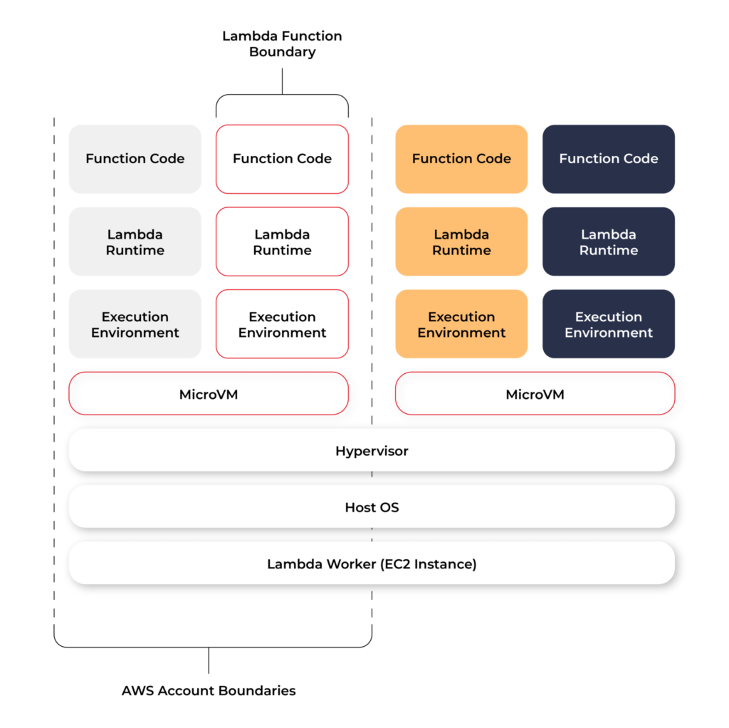
From an infrastructure standpoint, every AWS Lambda is part of a container running Amazon Linux (referenced as Function Container). The code files and assets you create for your AWS Lambda are called Function Code Package and are stored on an S3 bucket managed by AWS. Whenever a Lambda function is triggered, the Function Code Package is downloaded from the S3 bucket to the Function container and installed on its Lambda runtime environment. This process can be easily scaled, and multiple calls for a specific Lambda function can be performed without any trouble by the AWS infrastructure.
The Lambda service is divided into two control planes. The control plane is a master component responsible for making global decisions about provisioning, maintaining, and distributing a workload. A second plane is a data plane that controls the Invoke API that runs Lambda functions. When a Lambda function is invoked, the data plane allocates an execution environment to that function, chooses an existing execution environment that has already been set up for that function, then runs the function code in that environment.
Each function runs in one or more dedicated execution environments that are used for the lifetime of the function and then destroyed. Each execution environment hosts one concurrent invocation but is reused in place across multiple serial invocations of the same function. Execution environments run on hardware virtualized virtual machines (microVMs). A micro VM is dedicated to an AWS account but can be reused by execution environments across functions within an account. MicroVMs are packed onto an AWS-owned and managed hardware platform (Lambda Workers). Execution environments are never shared across functions and microVMs are never shared across AWS accounts.
Even though Lambda execution environments are never reused across functions, a single execution environment can be reused for invoking the same function, potentially existing for hours before it is destroyed.
Each Lambda execution environment also includes a writeable file system, available at /tmp . This storage is not accessible to other execution environments. As with the process state, files are written to /tmp remain for the lifetime of the execution environment.
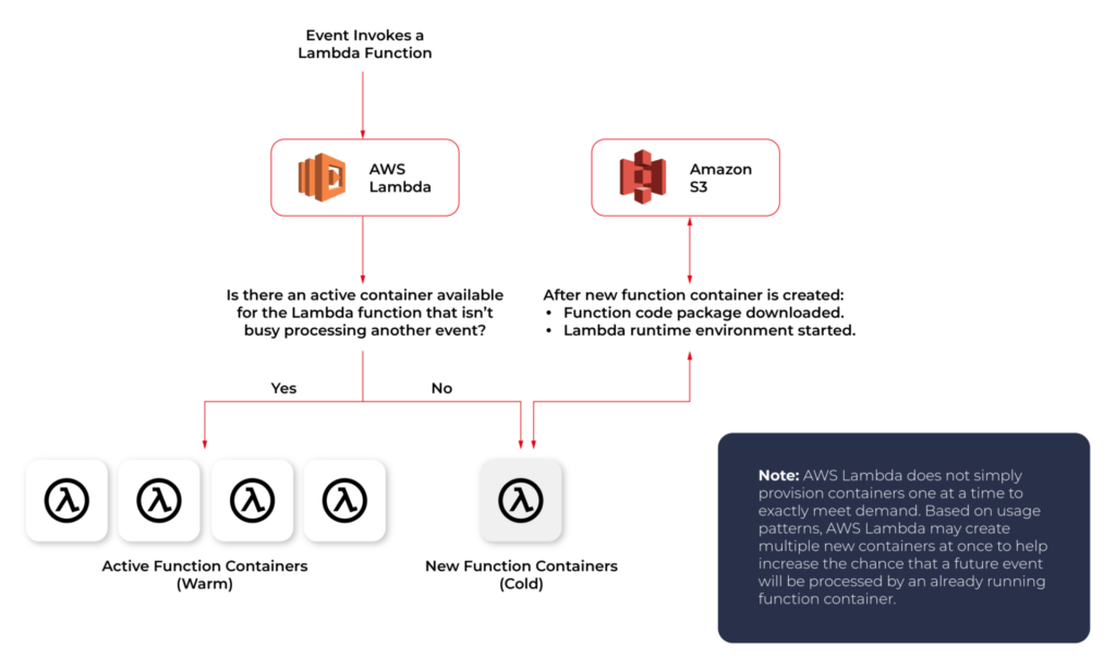
Cold start VS Warm start
When you call a Lambda Function, it follows the steps described above and executes the code. After finishing the execution, the Lambda Container stays available for a few minutes, before being terminated. This is called a Cold Start.
If you call the same function and the Lambda Container is still available (haven’t been terminated yet), AWS uses this container to execute your new call. This process of using active function containers is called Warm Container and it increases the response speed of your Lambda.
Role of AWS Lambda in serverless applications
There are a lot of use cases you can use AWS Lambda for, but there are killer cases for which Lambda is best suited:
- Operating serverless back-end
The web frontend can send requests to Lambda functions via API Gateway HTTPS endpoints. Lambda can handle the application logic and persist data to a fully-managed database service (RDS for relational, or DynamoDB for a non-relational database).
- Working with external services
If your application needs to request services from an external provider, there's generally no reason why the code for the site or the main application needs to handle the details of the request and the response. In fact, waiting for a response from an external source is one of the main causes of slowdowns in web-based services. If you hand requests for such things as credit authorization or inventory checks to an application running on AWS Lambda, your main program can continue with other elements of the transaction while it waits for a response from the Lambda function. This means that in many cases, a slow response from the provider will be hidden from your customers, since they will see the transaction proceeding, with the required data arriving and being processed before it closes.
- Near-realtime notifications
Any type of notifications, but particularly real-time, will find a use case with serverless Lambda. Once you create an SNS, you can set triggers that fire under certain policies. You can easily build a Lambda function to check log files from Cloudtrail or Cloudwatch. Lambda can search in the logs looking for specific events or log entries as they occur and send out notifications via SNS. You can also easily implement custom notification hooks to Slack or another system by calling its API endpoint within Lambda.
- Scheduled tasks and automated backups
Scheduled Lambda events are great for housekeeping within AWS accounts. Creating backups, checking for idle resources, generating reports, and other tasks which frequently occur can be implemented using AWS Lambda.
- Bulk real-time data processing
There are some cases when your application may need to handle large volumes of streaming input data, and moving that data to temporary storage for later processing may not be an adequate solution.If you send the data stream to an AWS Lambda application designed to quickly pull and process the required information, you can handle the necessary real-time tasks.
- Processing uploaded S3 objects
By using S3 object event notifications, you can immediately start processing your files by Lambda, once they land in S3 buckets. Image thumbnail generation with AWS Lambda is a great example for this use case, the solution will be cost-effective and you don’t need to worry about scaling up - Lambda will handle any load.
AWS Lambda limitations
AWS Lambda is not a silver bullet for every use case. For example, it should not be used for anything that you need to control or manage at the infrastructure level, nor should it be used for a large monolithic application or suite of applications.
Lambda comes with a number of “limitations”, which is good to keep in mind when architecting a solution.
There are some “hard limitations” for the runtime environment: the disk space is limited to 500MB, memory can vary from 128MB to 3GB and the execution timeout for a function is 15 minutes. Package constraints like the size of the deployment package (250MB) and the number of file descriptors (1024) are also defined as hard limits.
Similarly, there are “limitations” for the requests served by Lambda: request and response body synchronous event payload can be a maximum of 6 MB while an asynchronous invocation payload can be up to 256KB. At the moment, the only soft “limitation”, which you can request to be increased, is the number of concurrent executions, which is a safety feature to prevent any accidental recursive or infinite loops from going wild in the code. This would throttle the number of parallel executions.
All these limitations come from defined architectural principles for the Lambda service:
- If your Lambda function is running for hours, it should be moved to EC2 rather than Lambda.
- If the deployment package jar is greater than 50 MB in size, it should be broken down into multiple packages and functions.
- If the request payloads exceed the limits, you should break them up into multiple request endpoints.
It all comes down to preventing deploying monolithic applications as Lambda functions and designing stateless microservices as a collection of functions instead. Having this mindset, the “limitations” make complete sense.
AWS Lambda examples
Let’s now take a look at some AWS Lambda examples. We will start with a dummy Java application and how to create, deploy and trigger AWS Lambda. We will use AWS Command Line Interface(AWS CLI) to manage functions and other AWS Lambda resources.
Basic application
Let’s get started by creating the Lambda function and needed roles for Lambda execution.

This trust policy allows Lambda to use the role's permissions by giving the service principal lambda.amazonaws.com permission to call the AWS Security Token Service AssumeRole action. The content of trust-policy.json is the following:

Then let’s attach some permissions to the created role. To add permissions to the role, use the attach-policy-to-role command. Start by adding the AWSLambdaBasicExecutionRole managed policy.

Function code
As an example, we will create Java 11 application using Maven.
For Java AWS Lambda provides the following libraries:
- com.amazonaws:aws-lambda-java-core – Defines handler method interfaces and the context object that the runtime passes to the handler. This is a required library.
- com.amazonaws:aws-lambda-java-events – Different input types for events from services that invoke Lambda functions.
- com.amazonaws:aws-lambda-java-log4j2 – An appender library for Apache Log4j 2 that you can use to add the request ID for the current invocation to your function logs.
Let’s add Java core library to Maven application:

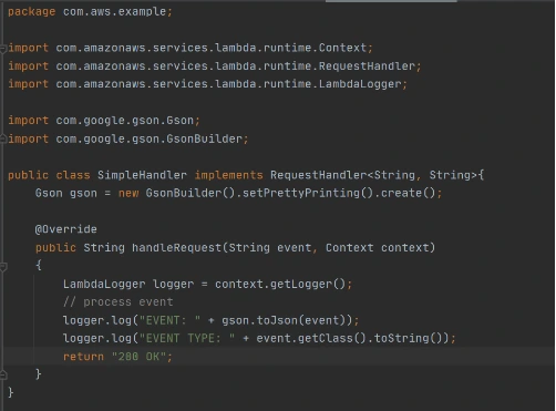
Then we need to add a Handler class which will be an entry point for our function. For Java function this Handler class should implement com.amazonaws.services.lambda.runtime.RequestHandler interface. It’s also possible to set generic input and output types.
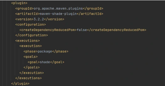
Now let’s create a deployment package from the source code. For Lambda deployment package should be either .zip or .jar. To build a jar file with all dependencies let’s use maven-shade-plugin .
After running mvn package command, the resulting jar will be placed into target folder. You can take this jar file and zip it.
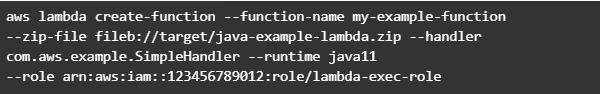
Now let’s create Lambda function from the generated deployment package.
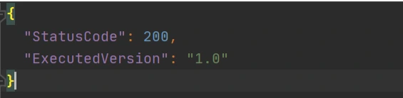
Once Lambda function is deployed we can test it. For that let’s use invoke-command.

out.json means the filename where the content will be saved. After invoking Lambda you should be able to see a similar result in your out.json :
More complicated example
Now let’s take a look at a more complicated application that will show the integration between several AWS services. Also, we will show how Lambda Layers can be used in function code. Let’s create an application with API Gateway as a proxy, two Lambda functions as some back-end logic, and DynamoDB as data storage. One Lambda will be intended to save a new record into the database. The second Lambda will be used to retrieve an object from the database by its identifier.
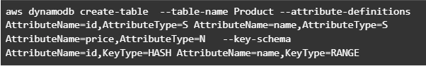
Let’s start by creating a table in DynamoDB. For simplicity, we’ll add just a couple of fields to that table.
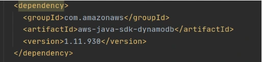
Now let’s create a Java module where some logic with database operations will be put. Dependencies to AWS DynamoDB SDK should be added to the module.
Now let’s add common classes and models to work with the database. This code will be reused in both lambdas.
Model entity object:
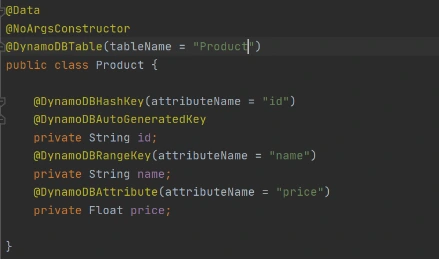
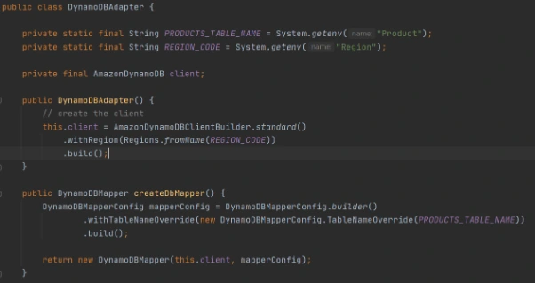
Adapter class to DynamoDB client.
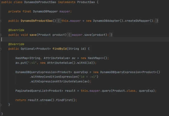
Implementation of DAO interface to provide needed persistent operations.
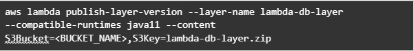
Now let’s build this module and package it into a jar with dependencies. From that jar, a reusable Lambda Layer will be created. Compress fat jar file as a zip archive and publish it to S3. After doing that we will be able to create a Lambda Layer.
Layer usage permissions are managed on the resource. To configure a Lambda function with a layer, you need permission to call GetLayerVersion on the layer version. For functions in your account, you can get this permission from your user policy or from the function's resource-based policy. To use a layer in another account, you need permission on your user policy, and the owner of the other account must grant your account permission with a resource-based policy.
Function code
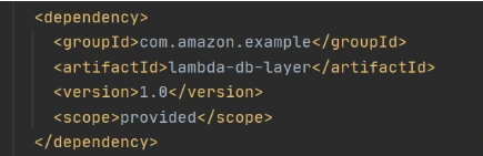
Now let’s add this shared dependency to both Lambda functions. To do that we need to define a provided dependency in pom.xml.
After that, we can write Lambda handlers. The first one will be used to persist new objects into the database:
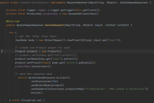
NOTE : in case of subsequent calls AWS may reuse the old Lambda instance instead of creating a new one. This offers some performance advantages to both parties: Lambda gets to skip the container and language initialization, and you get to skip initialization in your code. That’s why it’s recommended not to put the creation and initialization of potentially reusable objects into the handler body, but to move it to some code blocks which will be executed once - on the initialization step only.
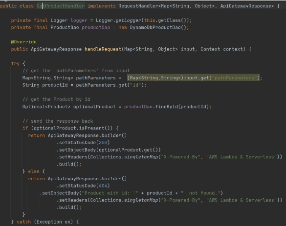
In the second Lambda function we will extract object identifiers from request parameters and fetch records from the database by id:
Now create Lambda functions as it was shown in the previous example. Then we need to configure layer usage for functions. To add layers to your function, use the update-function-configuration command.
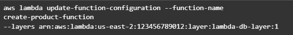
You must specify the version of each layer to use by providing the full Amazon Resource Name (ARN) of the layer version. While your function is running, it can access the content of the layer in the /opt directory. Layers are applied in the order that's specified, merging any folders with the same name. If the same file appears in multiple layers, the version in the last applied layer is used.
After attaching the layer to Lambda we can deploy and run it.
Now let’s create and configure API Gateway as a proxy to Lambda functions.

This operation will return json with the identifier of created API. Save the API ID for use in further commands. You also need the ID of the API root resource. To get the ID, run the get-resources command.

Now we need to create a resource that will be associated with Lambda to provide integration with functions.

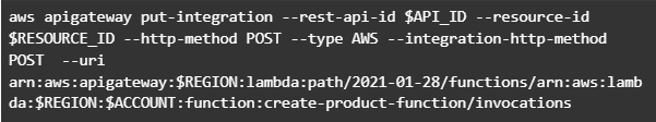
Parameter --integration-http-method is the method that API Gateway uses to communicate with AWS Lambda. Parameter --uri is a unique identifier for the endpoint to which Amazon API Gateway can send requests.
Now let’s make similar operations for the second lambda( get-by-id-function ) and deploy an API.

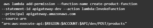
Note. Before testing API Gateway, you need to add permissions so that Amazon API Gateway can invoke your Lambda function when you send HTTP requests.
Now let’s test our API. First of all, we’ll try to add a new product record:

The result of this call will be like this:

Now we can retrieve created object by its identifier:
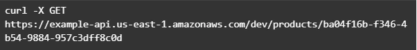
And you will get a similar result as after POST request. The same object will be returned in this example.
AWS Lambda tips
Debugging Lambda locally
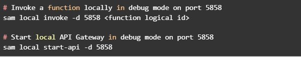
You can use AWS SAM console with a number of AWS toolkits to test and debug your serverless applications locally. For example, you can perform step-through debugging of your Lambda functions. The commands sam local invoke and sam local start-api both support local step-through debugging of your Lambda functions. To run AWS SAM locally with step-through debugging support enabled, specify --debug-port or -d on the command line. For example:
Also for debugging purposes, you can use AWS toolkits which are plugins that provide you with the ability to perform many common debugging tasks, like setting breakpoints, executing code line by line, and inspecting the values of variables. Toolkits make it easier for you to develop, debug, and deploy serverless applications that are built using AWS.
Configure CloudWatch monitoring and alerts
Lambda automatically monitors Lambda functions on your behalf and reports metrics through Amazon CloudWatch. To help you monitor your code when it runs, Lambda automatically tracks the number of requests, the invocation duration per request, and the number of requests that result in an error. Lambda also publishes the associated CloudWatch metrics. You can leverage these metrics to set CloudWatch custom alarms. The Lambda console provides a built-in monitoring dashboard for each of your functions and applications. Each time your function is invoked, Lambda records metrics for the request, the function's response, and the overall state of the function. You can use metrics to set alarms that are triggered when function performance degrades, or when you are close to hitting concurrency limits in the current AWS Region.
Beware of concurrency limits
For those functions whose usage scales along with your application traffic, it’s important to note that AWS Lambda functions are subject to concurrency limits. When functions reach 1,000 concurrent executions, they are subject to AWS throttling rules. Future calls will be delayed until your concurrent execution averages are back below the threshold. This means that as your applications scale, your high-traffic functions are likely to see drastic reductions in throughput during the time you need them most. To work around this limit, simply request that AWS raise your concurrency limits for the functions that you expect to scale.
Also, there are some widespread issues you may face working with Lambda:
Limitations while working with database
If you have a lot of reading/writing operations during one Lambda execution, you may probably face some failures due to Lambda limitations. Often the case is a timeout on Lambda execution. To investigate the problem you can temporarily increase the timeout limit on the function, but a common and highly recommended solution is to use batch operations while working with the database.
Timeout issues on external calls
This case may occur if you call a remote API from Lambda that takes too long to respond or that is unreachable. Network issues can also cause retries and duplicated API requests. To prepare for these occurrences, your Lambda function must always be idempotent. If you make an API call using an AWS SDK and the call fails, the SDK automatically retries the call. How long and how many times the SDK retries is determined by settings that vary among each SDK. To fix the retry and timeout issues, review the logs of the API call to find the problem. Then, change the retry count and timeout settings of the SDK as needed for each use case. To allow enough time for a response to the API call, you can even add time to the Lambda function timeout setting.
VPC connection issues
Lambda functions always operate from an AWS-owned VPC. By default, your function has full ability to make network requests to any public internet address — this includes access to any of the public AWS APIs. You should configure your functions for VPC access when you need to interact with a private resource located in a private subnet. When you connect a function to a VPC, all outbound requests go through your VPC. To connect to the internet, configure your VPC to send outbound traffic from the function's subnet to a NAT gateway in a public subnet.
Exploring Texas Instruments Edge AI: Hardware acceleration for efficient computation
In recent years, the field of artificial intelligence (AI) has witnessed a transformative shift towards edge computing, enabling intelligent decision-making to occur directly on devices rather than relying solely on cloud-based solutions. Texas Instruments, a key player in the semiconductor industry, has been at the forefront of developing cutting-edge solutions for Edge AI. One of the standout features of their offerings is the incorporation of hardware acceleration for efficient computation, which significantly improves the performance of AI models on resource-constrained devices.
Pros and cons of running AI models on embedded devices vs. cloud
In the evolving landscape of artificial intelligence , the decision to deploy models on embedded devices or rely on cloud-based solutions is a critical consideration. This chapter explores the advantages and disadvantages of running AI models on embedded devices, emphasizing the implications for efficiency, privacy, latency, and overall system performance.
Advantages of embedded AI
- Low Latency
One of the primary advantages of embedded AI is low latency. Models run directly on the device, eliminating the need for data transfer to and from the cloud. This results in faster response times, making embedded AI ideal for applications where real-time decision-making is crucial. - Privacy and Security
Embedded AI enhances privacy by processing data locally on the device. This mitigates concerns related to transmitting sensitive information to external servers. Security risks associated with data in transit are significantly reduced, contributing to a more secure AI deployment. - Edge Computing Efficiency
Utilizing embedded AI aligns with the principles of edge computing. By processing data at the edge of the network, unnecessary bandwidth usage is minimized, and only relevant information is transmitted to the cloud. This efficiency is especially beneficial in scenarios with limited network connectivity. What’s more, some problems are very inefficient to solve on cloud-based AI models, for example: video processing with real time output. - Offline Functionality
Embedded AI allows for offline functionality, enabling devices to operate independently of internet connectivity. This feature is advantageous in remote locations or environments with intermittent network access, as it expands the range of applications for embedded AI. - Reduced Dependence on Network Infrastructure
Deploying AI models on embedded devices reduces dependence on robust network infrastructure. This is particularly valuable in scenarios where maintaining a stable and high-bandwidth connection is challenging or cost ineffective. AI feature implemented on the cloud platform will be unavailable in the car after the connection is lost.
Disadvantages of embedded AI
- Lack of Scalability
Scaling embedded AI solutions across a large number of devices can be challenging. Managing updates, maintaining consistency, and ensuring uniform performance becomes more complex as the number of embedded devices increases. - Maintenance Challenges
Updating and maintaining AI models on embedded devices can be more cumbersome compared to cloud-based solutions. Remote updates may be limited, requiring physical intervention for maintenance, which can be impractical in certain scenarios. - Initial Deployment Cost
The initial cost of deploying embedded AI solutions, including hardware and development, can be higher compared to cloud-based alternatives. However, this cost may be offset by long-term benefits, depending on the specific use case and scale. - Limited Computational Power
Embedded devices often have limited computational power compared to cloud servers. This constraint may restrict the complexity and size of AI models that can be deployed on these devices, impacting the range of applications they can support. - Resource Constraints
Embedded devices typically have limited memory and storage capacities. Large AI models may struggle to fit within these constraints, requiring optimization or compromising model size for efficient deployment.
The decision to deploy AI models on embedded devices or in the cloud involves careful consideration of trade-offs. While embedded AI offers advantages in terms of low latency, privacy, and edge computing efficiency, it comes with challenges related to scalability, maintenance, and limited resources.
However, chipset manufacturers are constantly engaged in refining and enhancing their products by incorporating specialized modules dedicated to hardware-accelerated model execution. This ongoing commitment to innovation aims to significantly improve the overall performance of devices, ensuring that they can efficiently run AI models. The integration of these hardware-specific modules not only promises comparable performance but, in certain applications, even superior efficiency.
Deploy AI model on embedded device workflow
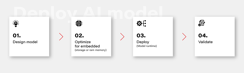
1. Design Model
Designing an AI model is the foundational step in the workflow. This involves choosing the appropriate model architecture based on the task at hand, whether it's classification, regression, or other specific objectives. This is out of the topic for this article.
2. Optimize for Embedded (Storage or RAM Memory)
Once the model is designed, the next step is to optimize it for deployment on embedded devices with limited resources. This optimization may involve reducing the model size, minimizing the number of parameters, or employing quantization techniques to decrease the precision of weights. The goal is to strike a balance between model size and performance to ensure efficient operation within the constraints of embedded storage and RAM memory.
3. Deploy (Model Runtime)
Deploying the optimized model involves integrating it into the embedded system's runtime environment. While there are general-purpose runtime frameworks like TensorFlow Lite and ONNX Runtime, achieving the best performance often requires leveraging dedicated frameworks that utilize hardware modules for accelerated computations. These specialized frameworks harness hardware accelerators to enhance the speed and efficiency of the model on embedded devices.
4. Validate
Validation is a critical stage in the workflow to ensure that the deployed model performs effectively on the embedded device. This involves rigorous testing using representative datasets and scenarios. Metrics such as accuracy, latency, and resource usage should be thoroughly evaluated to verify that the model meets the performance requirements. Validation helps identify any potential issues or discrepancies between the model's behavior in the development environment and its real-world performance on the embedded device.
Deploy model on Ti Edge AI and Jacinto 7
Deploying an AI model on Ti Edge AI and Jacinto 7 involves a series of steps to make the model work efficiently with both regular and specialized hardware. In simpler terms, we'll walk through how the model file travels from a general Linux environment to a dedicated DSP core, making use of special hardware features along the way.
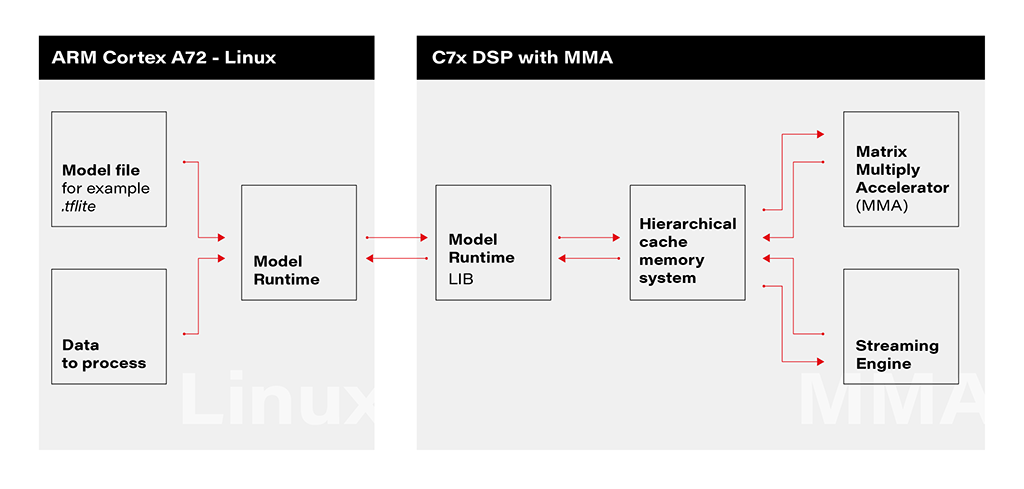
1. Linux Environment on A72 Core: The deployment process initiates within the Linux environment running on the A72 core. Here, a model file resides, ready to be utilized by the application's runtime. The model file, often in a standardized format like .tflite, serves as the blueprint for the AI model's architecture and parameters.
2. Runtime Application on A72 Core: The runtime application, responsible for orchestrating the deployment, receives the model file from the Linux environment. This runtime acts as a proxy between the user, the model, and the specialized hardware accelerator. It interfaces with the Linux environment, handling the transfer of input data to be processed by the model.
3. Connection to C7xDSP Core: The runtime application establishes a connection with its library executing on the C7xDSP core. This library, finely tuned for hardware acceleration, is designed to efficiently process AI models using specialized modules such as the Matrix Multiply Accelerator.
4. Loading Model and Data into Memory: The library on the C7x DSP core receives the model description and input data, loading them into memory for rapid access. This optimized memory utilization is crucial for achieving efficient inference on the dedicated hardware.
5. Computation with Matrix Multiply Accelerator: Leveraging the power of the Matrix Multiply Accelerator, the library performs the computations necessary for model inference. The accelerator efficiently handles matrix multiplications, a fundamental operation in many neural network models.
The matrix multiply accelerator (MMA) provides the following key features:
- Support for a fully connected layer using matrix multiply with arbitrary dimension
- Support for convolution layer using 2D convolution with matrix multiply with read panel Support for ReLU non-linearity layer OTF
- Support for high utilization (>85%) for a typical convolutional neural network (CNN), such as AlexNet, ResNet, and others
- Ability to support any CNN network topologies limited only by memory size and bandwidth
6. Result Return to User via Runtime on Linux: Upon completion of computations, the results are returned to the user through the runtime application on the Linux environment. The inference output, processed with hardware acceleration, provides high-speed, low-latency responses for real-time applications.
Object recognition with AI model on Jacinto 7: Real-world challenges
In this chapter, we explore a practical example of deploying an AI model on Jacinto 7 for object recognition. The model is executed according to the provided architecture, utilizing the TVM-CL-3410-gluoncv-mxnet-mobv2 model from the Texas Instruments Edge AI Model Zoo. The test images capture various scenarios, showcasing both successful and challenging object recognition outcomes.
The deployment architecture aligns with the schematic provided, incorporating Jacinto 7's capabilities to efficiently execute the AI model. The TVM-CL-3410-gluoncv-mxnet-mobv2 model is utilized, emphasizing its pre-trained nature for object recognition tasks.
Test Scenarios: A series of test images were captured to evaluate the model's performance in real-world conditions. Notably:

Challenges and Real-world Nuances: The test results underscore the challenges of accurate object recognition in less-than-ideal conditions. Factors such as image quality, lighting, and ambiguous object appearances contribute to the intricacy of the task. The third and fourth images, where scissors are misidentified as a screwdriver, and a Coca-Cola glass is misrecognized as wine, exemplify situations where even a human might face difficulty due to limited visual information-
Quality Considerations: The achieved results are noteworthy, considering the less-than-optimal quality of the test images. The chosen camera quality and lighting conditions intentionally mimic challenging real-world scenarios, making the model's performance commendable.
Conclusion: The real-world example of object recognition on Jacinto 7 highlights the capabilities and challenges associated with deploying AI models in practical scenarios. The successful identification of objects like a screwdriver, cup, and computer mouse demonstrates the model's efficacy. However, misidentifications in challenging scenarios emphasize the need for continuous refinement and adaptation, acknowledging the intricacies inherent in object recognition tasks, especially in dynamic and less-controlled environments.
How to run Selenium BDD tests in parallel with AWS Lambda
Have you ever felt annoyed because of the long waiting time for receiving test results? Maybe after a few hours, you’ve figured out that there had been a network connection issue in the middle of testing, and half of the results can go to the trash? That may happen when your tests are dependent on each other or when you have plenty of them and execution lasts forever. It's quite a common issue. But there’s actually a solution that can not only save your time but also your money - parallelization in the Cloud.
How it started
Developing UI tests for a few months, starting from scratch, and maintaining existing tests, I found out that it has become something huge that will be difficult to take care of very soon. An increasing number of test scenarios made every day led to bottlenecks. One day when I got to the office, it turned out that the nightly tests were not over yet. Since then, I have tried to find a way to avoid such situations.
A breakthrough was the presentation of Tomasz Konieczny during the Testwarez conference in 2019. He proved that it’s possible to run Selenium tests in parallel using AWS Lambda. There’s actually one blog that helped me with basic Selenium and Headless Chrome configuration on AWS. The Headless Chrome is a light-weighted browser that has no user interface. I went a step forward and created a solution that allows designing tests in the Behavior-Driven Development process and using the Page Object Model pattern approach, run them in parallel, and finally - build a summary report.
Setting up the project
The first thing we need to do is signing up for Amazon Web Services. Once we have an account and set proper values in credentials and config files (.aws directory), we can create a new project in PyCharm, Visual Studio Code, or in any other IDE supporting Python. We’ll need at least four directories here. We called them ‘lambda’, ‘selenium_layer’, ‘test_list’, ‘tests’ and there’s also one additional - ‘driver’, where we keep a chromedriver file, which is used when running tests locally in a sequential way.
In the beginning, we’re going to install the required libraries. Those versions work fine on AWS, but you can check newer if you want.
requirements.txt
allure_behave==2.8.6
behave==1.2.6
boto3==1.10.23
botocore==1.13.23
selenium==2.37.0
What’s important, we should install them in the proper directory - ‘site-packages’.
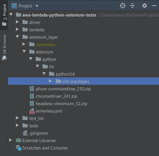
We’ll need also some additional packages:
Allure Commandline ( download )
Chromedriver ( download )
Headless Chromium ( download )
All those things will be deployed to AWS using Serverless Framework, which you need to install following the docs . The Serverless Framework was designed to provision the AWS Lambda Functions, Events, and infrastructure Resources safely and quickly. It translates all syntax in serverless.yml to a single AWS CloudFormation template which is used for deployments.
Architecture - Lambda Layers
Now we can create a serverless.yml file in the ‘selenium-layer’ directory and define Lambda Layers we want to create. Make sure that your .zip files have the same names as in this file. Here we can also set the AWS region in which we want to create our Lambda functions and layers.
serverless.yml
service: lambda-selenium-layer
provider:
name: aws
runtime: python3.6
region: eu-central-1
timeout: 30
layers:
selenium:
path: selenium
CompatibleRuntimes: [
"python3.6"
]
chromedriver:
package:
artifact: chromedriver_241.zip
chrome:
package:
artifact: headless-chromium_52.zip
allure:
package:
artifact: allure-commandline_210.zip
resources:
Outputs:
SeleniumLayerExport:
Value:
Ref: SeleniumLambdaLayer
Export:
Name: SeleniumLambdaLayer
ChromedriverLayerExport:
Value:
Ref: ChromedriverLambdaLayer
Export:
Name: ChromedriverLambdaLayer
ChromeLayerExport:
Value:
Ref: ChromeLambdaLayer
Export:
Name: ChromeLambdaLayer
AllureLayerExport:
Value:
Ref: AllureLambdaLayer
Export:
Name: AllureLambdaLayer
Within this file, we’re going to deploy a service consisting of four layers. Each of them plays an important role in the whole testing process.
Creating test set
What would the tests be without the scenarios? Our main assumption is to create test files running independently. This means we can run any test without others and it works. If you're following clean code, you'll probably like using the Gherkin syntax and the POM approach. Behave Framework supports both.
What gives us Gherkin? For sure, better readability and understanding. Even if you haven't had the opportunity to write tests before, you will understand the purpose of this scenario.
01.OpenLoginPage.feature
@smoke
@login
Feature: Login to service
Scenario: Login
Given Home page is opened
And User opens Login page
When User enters credentials
And User clicks Login button
Then User account page is opened
Scenario: Logout
When User clicks Logout button
Then Home page is opened
And User is not authenticated
In the beginning, we have two tags. We add them in order to run only chosen tests in different situations. For example, you can name a tag @smoke and run it as a smoke test, so that you can test very fundamental app functions. You may want to test only a part of the system like end-to-end order placing in the online store - just add the same tag for several tests.
Then we have the feature name and two scenarios. Those are quite obvious, but sometimes it’s good to name them with more details. Following steps starting with Given, When, Then and And can be reused many times. That’s the Behavior-Driven Development in practice. We’ll come back to this topic later.
Meantime, let’s check the proper configuration of the Behave project.
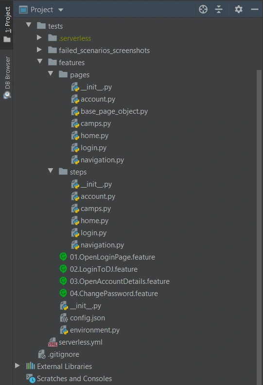
We definitely need a ‘feature’ directory with ‘pages’ and ‘steps’. Make the ‘feature’ folder as Sources Root. Just right-click on it and select the proper option. This is the place for our test scenario files with .feature extension.
It’s good to have some constant values in a separate file so that it will change only here when needed. Let’s call it config.json and put the URL of the tested web application.
config.json
{
"url": "http://drabinajakuba.atthost24.pl/"
}
One more thing we need is a file where we set webdriver options.
Those are required imports and some global values like, e.g. a name of AWS S3 bucket in which we want to have screenshots or local directory to store them in. As far as we know, bucket names should be unique in whole AWS S3, so you should probably change them but keep the meaning.
environment.py
import os
import platform
from datetime import date, datetime
import json
import boto3
from selenium import webdriver
from selenium.webdriver.chrome.options import Options
REPORTS_BUCKET = 'aws-selenium-test-reports'
SCREENSHOTS_FOLDER = 'failed_scenarios_screenshots/'
CURRENT_DATE = str(date.today())
DATETIME_FORMAT = '%H_%M_%S'
Then we have a function for getting given value from our config.json file. The path of this file depends on the system platform - Windows or Darwin (Mac) would be local, Linux in this case is in AWS. If you need to run these tests locally on Linux, you should probably add some environment variables and check them here.
def get_from_config(what):
if 'Linux' in platform.system():
with open('/opt/config.json') as json_file:
data = json.load(json_file)
return data[what]
elif 'Darwin' in platform.system():
with open(os.getcwd() + '/features/config.json') as json_file:
data = json.load(json_file)
return data[what]
else:
with open(os.getcwd() + '\\features\\config.json') as json_file:
data = json.load(json_file)
return data[what]
Now we can finally specify paths to chromedriver and set browser options which also depend on the system platform. There’re a few more options required on AWS.
def set_linux_driver(context):
"""
Run on AWS
"""
print("Running on AWS (Linux)")
options = Options()
options.binary_location = '/opt/headless-chromium'
options.add_argument('--allow-running-insecure-content')
options.add_argument('--ignore-certificate-errors')
options.add_argument('--disable-gpu')
options.add_argument('--headless')
options.add_argument('--window-size=1280,1000')
options.add_argument('--single-process')
options.add_argument('--no-sandbox')
options.add_argument('--disable-dev-shm-usage')
capabilities = webdriver.DesiredCapabilities().CHROME
capabilities['acceptSslCerts'] = True
capabilities['acceptInsecureCerts'] = True
context.browser = webdriver.Chrome(
'/opt/chromedriver', chrome_options=options, desired_capabilities=capabilities
)
def set_windows_driver(context):
"""
Run locally on Windows
"""
print('Running on Windows')
options = Options()
options.add_argument('--no-sandbox')
options.add_argument('--window-size=1280,1000')
options.add_argument('--headless')
context.browser = webdriver.Chrome(
os.path.dirname(os.getcwd()) + '\\driver\\chromedriver.exe', chrome_options=options
)
def set_mac_driver(context):
"""
Run locally on Mac
"""
print("Running on Mac")
options = Options()
options.add_argument('--no-sandbox')
options.add_argument('--window-size=1280,1000')
options.add_argument('--headless')
context.browser = webdriver.Chrome(
os.path.dirname(os.getcwd()) + '/driver/chromedriver', chrome_options=options
)
def set_driver(context):
if 'Linux' in platform.system():
set_linux_driver(context)
elif 'Darwin' in platform.system():
set_mac_driver(context)
else:
set_windows_driver(context)
Webdriver needs to be set before all tests, and in the end, our browser should be closed.
def before_all(context):
set_driver(context)
def after_all(context):
context.browser.quit()
Last but not least, taking screenshots of test failure. Local storage differs from the AWS bucket, so this needs to be set correctly.
def after_scenario(context, scenario):
if scenario.status == 'failed':
print('Scenario failed!')
current_time = datetime.now().strftime(DATETIME_FORMAT)
file_name = f'{scenario.name.replace(" ", "_")}-{current_time}.png'
if 'Linux' in platform.system():
context.browser.save_screenshot(f'/tmp/{file_name}')
boto3.resource('s3').Bucket(REPORTS_BUCKET).upload_file(
f'/tmp/{file_name}', f'{SCREENSHOTS_FOLDER}{CURRENT_DATE}/{file_name}'
)
else:
if not os.path.exists(SCREENSHOTS_FOLDER):
os.makedirs(SCREENSHOTS_FOLDER)
context.browser.save_screenshot(f'{SCREENSHOTS_FOLDER}/{file_name}')
Once we have almost everything set, let’s dive into single test creation. Page Object Model pattern is about what exactly hides behind Gherkin’s steps. In this approach, we treat each application view as a separate page and define its elements we want to test. First, we need a base page implementation. Those methods will be inherited by all specific pages. You should put this file in the ‘pages’ directory.
base_page_object.py
from selenium.webdriver.common.action_chains import ActionChains
from selenium.webdriver.support.ui import WebDriverWait
from selenium.webdriver.support import expected_conditions as EC
from selenium.common.exceptions import *
import traceback
import time
from environment import get_from_config
class BasePage(object):
def __init__(self, browser, base_url=get_from_config('url')):
self.base_url = base_url
self.browser = browser
self.timeout = 10
def find_element(self, *loc):
try:
WebDriverWait(self.browser, self.timeout).until(EC.presence_of_element_located(loc))
except Exception as e:
print("Element not found", e)
return self.browser.find_element(*loc)
def find_elements(self, *loc):
try:
WebDriverWait(self.browser, self.timeout).until(EC.presence_of_element_located(loc))
except Exception as e:
print("Element not found", e)
return self.browser.find_elements(*loc)
def visit(self, url):
self.browser.get(url)
def hover(self, element):
ActionChains(self.browser).move_to_element(element).perform()
time.sleep(5)
def __getattr__(self, what):
try:
if what in self.locator_dictionary.keys():
try:
WebDriverWait(self.browser, self.timeout).until(
EC.presence_of_element_located(self.locator_dictionary[what])
)
except(TimeoutException, StaleElementReferenceException):
traceback.print_exc()
return self.find_element(*self.locator_dictionary[what])
except AttributeError:
super(BasePage, self).__getattribute__("method_missing")(what)
def method_missing(self, what):
print("No %s here!", what)
That’s a simple login page class. There’re some web elements defined in locator_dictionary and methods using those elements to e.g., enter text in the input, click a button, or read current values. Put this file in the ‘pages’ directory.
login.py
from selenium.webdriver.common.by import By
from .base_page_object import *
class LoginPage(BasePage):
def __init__(self, context):
BasePage.__init__(
self,
context.browser,
base_url=get_from_config('url'))
locator_dictionary = {
'username_input': (By.XPATH, '//input[@name="username"]'),
'password_input': (By.XPATH, '//input[@name="password"]'),
'login_button': (By.ID, 'login_btn'),
}
def enter_username(self, username):
self.username_input.send_keys(username)
def enter_password(self, password):
self.password_input.send_keys(password)
def click_login_button(self):
self.login_button.click()
What we need now is a glue that will connect page methods with Gherkin steps. In each step, we use a particular page that handles the functionality we want to simulate. Put this file in the ‘steps’ directory.
login.py
from behave import step
from environment import get_from_config
from pages import LoginPage, HomePage, NavigationPage
@step('User enters credentials')
def step_impl(context):
page = LoginPage(context)
page.enter_username('test_user')
page.enter_password('test_password')
@step('User clicks Login button')
def step_impl(context):
page = LoginPage(context)
page.click_login_button()
It seems that we have all we need to run tests locally. Of course, not every step implementation was shown above, but it should be easy to add missing ones.
If you want to read more about BDD and POM, take a look at Adrian’s article
All files in the ‘features’ directory will also be on a separate Lambda Layer. You can create a serverless.yml file with the content presented below.
serverless.yml
service: lambda-tests-layer
provider:
name: aws
runtime: python3.6
region: eu-central-1
timeout: 30
layers:
features:
path: features
CompatibleRuntimes: [
"python3.6"
]
resources:
Outputs:
FeaturesLayerExport:
Value:
Ref: FeaturesLambdaLayer
Export:
Name: FeaturesLambdaLayer
This is the first part of the series covering running Parallel Selenium tests on AWS Lambda. More here !
Interested in our services?
Reach out for tailored solutions and expert guidance.