Getting Started with The Julia Language

Are you looking for a programming language that is fast, easy to start with, and trending? The Julia language meets the requirements. In this article, we show you how to take your first steps.

What is the Julia language?

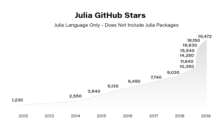
Julia is an open-source programming language for general purposes. However, it is mainly used for data science, machine learning, or numerical and statistical computing. It is gaining more and more popularity. According to the TIOBE index, the Julia language jumped from position 47 to position 23 in 2020 and is highly expected to head towards the top 20 next year.

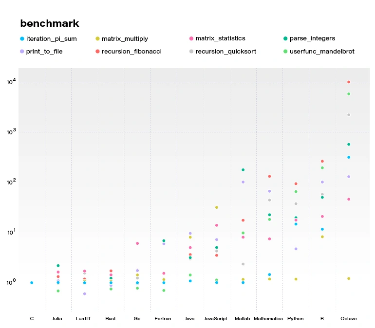
Despite the fact Julia is a flexible dynamic language, it is extremely fast. Well-written code is usually as fast as C, even though it is not a low-level language. It means it is much faster than languages like Python or R, which are used for similar purposes. High performance is achieved by using type interference and JIT (just-in-time) compilation with some AOT (ahead-of-time) optimizations. You can directly call functions from other languages such as C, C++, MATLAB, Python, R, FORTRAN… On the other hand, it provides poor support for static compilation, since it is compiled at runtime.

Julia makes it easy to express many object-oriented and functional programming patterns. It uses multiple dispatches, which is helpful, especially when writing a mathematical code. It feels like a scripting language and has good support for interactive use. All those attributes make Julia very easy to get started with and experiment with.

First steps with the Julina language

1. Download and install Julia from Download Julia.
2. (Optional – not required to follow the article) Choose your IDE for the Julia language. VS Code is probably the most advanced option available at the moment of writing this paragraph. We encourage you to do your research and choose one according to your preferences. To install VSCode, please follow Installing VS Code and VS Code Julia extension.

Playground

Let’s start with some experimenting in an interactive session. Just run the Julia command in a terminal. You might need to add Julia’s binary path to your PATH variable first. This is the fastest way to learn and play around with Julia.

C:\Users\prso\Desktop>julia
               _
   _       _ _(_)_     |  Documentation: https://docs.julialang.org
  (_)     | (_) (_)    |
   _ _   _| |_  __ _   |  Type "?" for help, "]?" for Pkg help.
  | | | | | | |/ _` |  |
  | | |_| | | | (_| |  |  Version 1.5.3 (2020-11-09)
 _/ |\__'_|_|_|\__'_|  |  Official https://julialang.org/ release
|__/                   |

julia> println("hello world")
hello world

julia> 2^10
1024

julia> ans*2
2048

julia> exit()

C:\Users\prso\Desktop>

To get a recently returned value, we can use the ans variable. To close REPL, use exit() function or Ctrl+D shortcut.

Running the scripts

You can create and run your scripts within an IDE. But, of course, there are more ways to do so. Let’s create our first script in any text editor and name it: example.jl.

x = 2
println(10x)

You can run it from REPL:

julia> include("example.jl")
20

Or, directly from your system terminal:

C:\Users\prso\Desktop>julia example.jl
20

Please be aware that REPL preserves the current state and includes statement works like a copy-paste. It means that running included is the equivalent of typing this code directly in REPL. It may affect your subsequent commands.

Basic types

Julia provides a broad range of primitive types along with standard mathematical functions and operators. Here’s the list of all primitive numeric types:

• Int8, UInt8
• Int16, UInt16
• Int32, UInt32
• Int64, UInt64
• Int128, UInt128
• Float16
• Float32
• Float64

A digit suffix implies several bits and a U prefix that is unsigned. It means that UInt64 is unsigned and has 64 bits. Besides, it provides full support for complex and rational numbers.

It comes with Bool, Char, and String types along with non-standard string literals such as Regex as well. There is support for non-ASCII characters. Both variable names and values can contain such characters. It can make mathematical expressions very intuitive.

julia> x = 'a'
'a': ASCII/Unicode U+0061 (category Ll: Letter, lowercase)

julia> typeof(ans)
Char

julia> x = 'β'
'β': Unicode U+03B2 (category Ll: Letter, lowercase)

julia> typeof(ans)
Char

julia> x = "tgα * ctgα = 1"
"tgα * ctgα = 1"

julia> typeof(ans)
String

julia> x = r"^[a-zA-z]{8}$"
r"^[a-zA-z]{8}$"

julia> typeof(ans)
Regex    

Storage: Arrays, Tuples, and Dictionaries

The most commonly used storage types in the Julia language are: arrays, tuples, dictionaries, or sets. Let’s take a look at each of them.

Arrays

An array is an ordered collection of related elements. A one-dimensional array is used as a vector or list. A two-dimensional array acts as a matrix or table. More dimensional arrays express multi-dimensional matrices.
Let’s create a simple non-empty array:

julia> a = [1, 2, 3]
3-element Array{Int64,1}:
 1
 2
 3

julia> a = ["1", 2, 3.0]
3-element Array{Any,1}:
  "1"
 2
 3.0

Above, we can see that arrays in Julia might store Any objects. However, this is considered an anti-pattern. We should store specific types in arrays for reasons of performance.

Another way to make an array is to use a Range object or comprehensions (a simple way of generating and collecting items by evaluating an expression).

julia> typeof(1:10)
UnitRange{Int64}

julia> collect(1:3)
3-element Array{Int64,1}:
 1
 2
 3

julia> [x for x in 1:10 if x % 2 == 0]
5-element Array{Int64,1}:
  2
  4
  6
  8
 10

We’ll stop here. However, there are many more ways of creating both one and multi-dimensional arrays in Julia.

There are a lot of built-in functions that operate on arrays. Julia uses a functional style unlike dot-notation in Python. Let’s see how to add or remove elements.

julia> a = [1,2]
2-element Array{Int64,1}:
 1
 2

julia> push!(a, 3)
3-element Array{Int64,1}:
 1
 2
 3

julia> pushfirst!(a, 0)
4-element Array{Int64,1}:
 0
 1
 2
 3

julia> pop!(a)
3

julia> a
3-element Array{Int64,1}:
 0
 1
 2

Tuples

Tuples work the same way as arrays. A tuple is an ordered sequence of elements. However, there is one important difference. Tuples are immutable. Trying to call methods like push!() will result in an error.

julia> t = (1,2,3)
(1, 2, 3)

julia> t[1]
1

Dictionaries

The next commonly used collections in Julia are dictionaries. A dictionary is called Dict for short. It is, as you probably expect, a key-value pair collection.
Here is how to create a simple dictionary:

julia> d = Dict(1 => "a", 2 => "b")
Dict{Int64,String} with 2 entries:
  2 => "b"
  1 => "a"

julia> d = Dict(x => 2^x for x = 0:5)
Dict{Int64,Int64} with 6 entries:
  0 => 1
  4 => 16
  2 => 4
  3 => 8
  5 => 32
  1 => 2

julia> sort(d)
OrderedCollections.OrderedDict{Int64,Int64} with 6 entries:
  0 => 1
  1 => 2
  2 => 4
  3 => 8
  4 => 16
  5 => 32

We can see, that dictionaries are not sorted. They don’t preserve any particular order. If you need that feature, you can use SortedDict.

julia> import DataStructures

julia> d = DataStructures.SortedDict(x => 2^x for x = 0:5)
DataStructures.SortedDict{Any,Any,Base.Order.ForwardOrdering} with 6 entries:
  0 => 1
  1 => 2
  2 => 4
  3 => 8
  4 => 16
  5 => 32

DataStructures is not an out-of-the-box package. To use it for the first time, we need to download it. We can do it with a Pkg package manager.

julia> import Pkg; Pkg.add("DataStructures")

Sets

Sets are another type of collection in Julia. Just like in many other languages, Set doesn’t preserve the order of elements and doesn’t store duplicated items. The following example creates a Set with a specified type and checks if it contains a given element.

julia> s = Set{String}(["one", "two", "three"])
Set{String} with 3 elements:
  "two"
  "one"
  "three"

julia> in("two", s)
true

This time we specified a type of collection explicitly. You can do the same for all the other collections as well.

Functions

Let’s recall what we learned about quadratic equations at school. Below is an example script that calculates the roots of a given equation: ax2+bx+c.

discriminant(a, b, c) = b^2 - 4a*c

function rootsOfQuadraticEquation(a, b, c)
    Δ = discriminant(a, b, c)
    if Δ > 0
        x1 = (-b - √Δ)/2a
        x2 = (-b + √Δ)/2a
        return x1, x2
    elseif Δ == 0
        return -b/2a
    else
        x1 = (-b - √complex(Δ))/2a
        x2 = (-b + √complex(Δ))/2a
        return x1, x2
    end
end

println("Two roots: ", rootsOfQuadraticEquation(1, -2, -8))
println("One root: ", rootsOfQuadraticEquation(2, -4, 2))
println("No real roots: ", rootsOfQuadraticEquation(1, -4, 5))

There are two functions. The first one is just a one-liner and calculates a discriminant of the equation. The second one computes the roots of the function. It returns either one value or multiple values using tuples.

We don’t need to specify argument types. The compiler checks those types dynamically. Please take note that the same happens when we call sqrt() function using a √ symbol. In that case, when the discriminant is negative, we need to wrap it with a complex()function to be sure that the sqrt() function was called with a complex argument.
Here is the console output of the above script:

C:\Users\prso\Documents\Julia>julia quadraticEquations.jl
Two roots: (-2.0, 4.0)
One root: 1.0
No real roots: (2.0 - 1.0im, 2.0 + 1.0im)

Plotting

Plotting with the Julia language is straightforward. There are several packages for plotting. We use one of them, Plots.jl.
To use it for the first, we need to install it:

julia> using Pkg; Pkg.add("Plots") 

After the package was downloaded, let’s jump straight to the example:

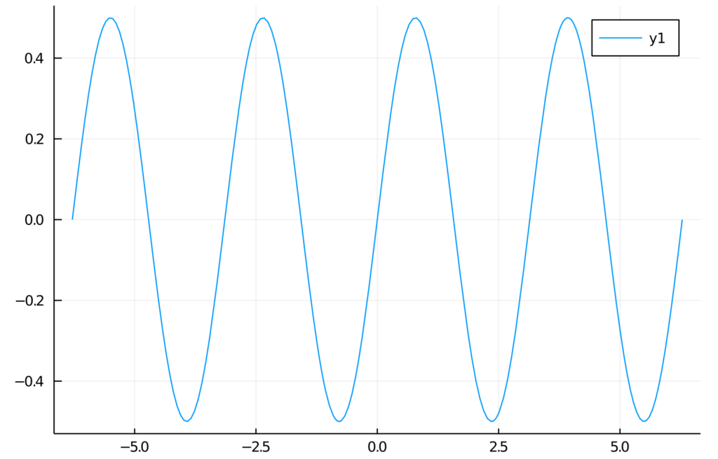
julia> f(x) = sin(x)cos(x)
f (generic function with 1 method)

julia> plot(f, -2pi, 2pi)

We’re expecting a graph of a function in a range from -2π to 2π. Here is the output:

Summary and further reading

In this article, we learned how to get started with Julia. We installed all the required components. Then we wrote our first “hello world” and got acquainted with basic Julia elements.

Of course, there is no way to learn a new language from reading one article. Therefore, we encourage you to play around with the Julia language on your own.

To dive deeper, we recommend reading the following sources:

• Official Getting Started Guide
• Introducing Julia in Wikibooks