Front note: This draft reflects A2A v1.0.1 and MCP 2025-11-25. Be aware of new versions available when reading this text.

Once upon a time, I had a presentation entitled “From Chatbot to AI Assistant”. It opened with an explanation of what this whole AI thing was about, followed by a funny (I believe) meme with Despicable Me’s Gru and boards that read: “we use state of the art frameworks, we follow official docs, we kill the application”. The central idea was a small diagram – request, look for data, answer – that gradually evolved into several modern AI-assistant architectures.

Well… the AI world moves at breakneck speed these days.

So, let me ask the same question again – how do you turn a simple chatbot into a useful AI assistant in mid-2026, and more importantly – why is last year’s approach already so outdated? A production assistant still depends on explicit orchestration, shared contracts, security boundaries, resilience and end-to-end observability. The answer boils down to two acronyms: MCP and A2A. Both have changed the default approach by standardizing two different seams in an agentic system.

New protocols: MCP and A2A explained

A year ago, there was no standard to organize agents, so every team tried to do it their own way. Plenty of solid assistants were built in those days, and many of them still serve customers to this day. Then, one day, the world went crazy about MCP (to be fair, the first version had been released even earlier). Model Context Protocol is a way to provide context for the model. The idea behind it is to unify tool calling and automate the provisioning of system prompts. The latter isn’t very useful, as you can use prompt management tools like Langfuse with staging tags instead, or any other system that fits your organization. Tool calling, on the other hand, used to be a nightmare. You, the developer, had to organize tool management (best case with live updates), parse LLM responses, extract parameters, pass them to tools and handle the loop back. There was a core “if” in the middle of the application to distinguish between an LLM answer to the user and an LLM request to execute some action or collect some data. With MCP, all you need to do is to provide the MCP server’s URL and then go grab a coffee while the work takes care of itself – the server maintainer takes care of tool descriptions and updates, and the SDK calls tools under the hood (I’ll return to this point in a moment).

Another new standard is the Agent-to-Agent protocol (A2A) – a standardized way for one agent to call another – complete with agent discovery, long polling, asynchronous responses, authorization and input requests, and streaming. A2A is a good fit when the remote component is an autonomous system that reasons, plans, maintains state, performs a multi-step task, or is owned and deployed independently. With A2A you can spin up an endless web of agents – each of them can call “something,” and this “something” might be another agent that could call the next one, which calls another, and another, and another…

Freedom! And you can create an assistant in a few hours!

But freedom never comes for free.

The first catch is the SDK-driven MCP tool calling mentioned above. When the LLM decides to call a tool, the entire request-response loop is executed automatically. It’s fast to develop, but there are three major drawbacks.

1. The monitoring capabilities are limited – OTel auto-instrumentation is the only way to see your tool calls in Langfuse, and you cannot really tweak the spans
2. You don’t control the request – if the LLM hallucinates, you can’t stop it. If the model has no access to some metadata (PII, for example), it won’t attach it.
3. You don’t process the response – if the tool returns extra information beyond the response itself (like a link to the source of the data), you need to rely on the LLM to process that metadata.

The second catch is A2A’s freedom. It’s the REST of the 21st century. With REST, you can cook up an endless spaghetti of services, but that doesn’t mean you should. With agents, it’s much easier to create an agent loop or exceed any acceptable response time than with regular services, so you need to design your application’s architecture with care.

New architecture: A three-layer MCP + A2A assistant

Let me ask one more time: how do you convert a simple chatbot into a useful AI assistant? The answer is: with MCP and A2A, but you need to use them wisely.

My proposal is a three-layer, tree-like structure – one or more entry-point agents that call working agents, which in turn call MCP servers with tools.

Bear in mind that this system can NOT work sequentially. All master agent LLM calls (see below), LLM-based agents and tool executions can take many seconds, so pay close attention to asynchronous processing in your application.

Master agent: The A2A entry-point

The first layer contains user-facing AI assistants – end-user exposed backend applications with simple REST/SSE endpoints to conduct conversations. As a rule, start with a single entry-point and make it flexible enough for different kinds of users; further down the line, however, it’s common to spin up more for specific use cases.

A master agent is an A2A client. It picks an agent and handles communication. But this is just the beginning. The core responsibility is to drive the conversation:

• execute named entity recognition (NER) to compute metadata from prompts,
• all multiple agents in parallel and verify the responses,
• react to “input-required” responses from agents and collect the required information using metadata or other agents,
• handle small talk on its own,
• verify requests and responses based on pre-defined rules,
• handle the tone and language of the conversation,
• produce intermediate messages like “I’m collecting data about your profile now”,
• implement circuit-breaker functionality so it never waits too long for hanging agents.

It also takes care of the technical side of things:

• enforce role-based access control
• send notifications for asynchronous responses
• prepare rich responses with all data returned from agents (media, closed-questions controllers, forms, etc.).

Working agents: Scaling out with A2A servers

The agent layer is how the system scales out. One team could own the entry-point, and then multiple teams might provide new agents to extend the system. Unfortunately, A2A is very flexible, so to keep the system maintainable and extensible in the long run, you need to lay down stricter requirements of your own. The schema of the DataPart field is key – there is no technical way to keep it consistent, so you need to enforce a company rule for that. You therefore need a common metadata schema across the system, so that one team doesn’t call the same piece of data “vehicle” while another calls it “model” and a third “vehicleModel” or even “vehicle_model”. You can start with an A2A extension covering:

• schema versions, required fields and compatibility rules;
• field names, meaning, units, locale and timestamp conventions;
• provenance and confidence for inferred or retrieved values;
• data classification, PII handling and redaction requirements;
• error categories and partial-result semantics; and
• conformance tests that every agent must pass before registration.

But at the end of the day, you need to validate the profile, as there is no enforcement in the protocol so far.

Keeping the metadata schema consistent lets every agent manage metadata, not just the entry-point – which comes in handy when a more specialized agent can recognize or obtain extra data that the whole assistant can put to use.

Building agents is usually very simple. It’s just an LLM-based application wrapped as an A2A server, with a prompt, an MCP integration and a bit of extra code to utilize all features of A2A – for example to send execution statuses (“planning”, “collecting data”, etc.) or rich responses. This approach significantly speeds up development and reduces the complexity of system components.

One caveat about the architecture. The diagram above shows a nice and clean one, but you never know when some team will slip agent-to-agent communication under the hood. That’s why you need a clock-based circuit breaker on the entry-point to avoid infinite (or merely very long) loops.

Tools: Wrapping capabilities in MCP servers

The MCP hype is sky-high these days. Everyone wants to wrap every available tool in an MCP server to make it AI-ready. That’s great, but “AI-ready”should not mean “placed behind a protocol without governance”.

SDK limitations: Using MCP structured content

Like A2A’s DataPart, MCP can return structuredContent instead of a plain-text response and carry more than words. By default, MCP-wrapped tools return plain text for LLMs, but there is usually far more worth returning, like discovered metadata or rich elements to show the customer (a document preview or a link). To make use of MCP’s structuredContent, you need to step back to the agents and replace the SDK-based MCP integration with custom code. There are two options. You can list the tools manually, build the LLM’s “tool calling” feature yourself and then execute the MCP calls on your own, or you can stand up MCP proxies alongside the agents. Then, when the LLM decides to call an MCP tool, the SDK hits a localhost server running inside the same process of the same application, and that proxy server calls the real, remote MCP. The proxy’s role is to enrich the request with authorization or metadata the LLM cannot handle (for consistency or legal reasons) and to deal with any extra fields that come back – forwarding them to the master agent, for example.

RBAC: Access control for MCP tools

The second challenge is access control. Usually, new agents with a limited set of capabilities can be protected in binary fashion – either a user has access or they don’t. But when it comes to existing REST-based services – with their sprawling capabilities, complex data classification and high-impact actions – nobody in their right mind would hand an LLM the keys.

But there is no need to reinvent the wheel here. You can simply add a custom header to MCP calls and verify user permissions at two points – when listing tools and when executing them. For that I recommend OAuth 2.0 Token Exchange with token caching, but if you would rather avoid extra round trips to the IdP, you might consider passing tokens through as-is between layers (strongly discouraged, and in fact forbidden by MCP, but still common).

Monitoring: Observability with Langfuse and OpenTelemetry

One of the nicest things about a monolithic agentic application, such as one built with LangGraph, is how observable the flow is. Being able to see the application’s steps as a diagram or a Gantt chart – and to debug every agent and tool in one place – is worth its weight in gold.

With a multi-layer, multi-agent, multi-tool application you can achieve the same, but it takes some discipline. Each component should have its own Langfuse integration and report new observations against the parent observation. That means every component calling a downstream one has to pass its own observation ID as metadata on the request to the other application. Keep an eye on clock synchronization between your servers, and voilà! Every single trace in Langfuse then tells the whole story of what happened, neatly laid out.

Unfortunately, so far Langfuse offers no mechanism to grant write-only access, so you end up spreading a key with far too many permissions across your application, but this issue is already under discussion and hopefully will be fixed soon. In the meantime, you can restrict the key to POST requests only, at the network layer of your infrastructure.

Also, MCP is becoming more aware of the issue. The new version 2026-07-28 documents traceparent, tracestate and baggage propagation in request metadata, allowing a tool call to appear in one OpenTelemetry-compatible trace, but it is still a release candidate, so this article is based on the previous version.

Demo: A multi-agent AI assistant in action

The demo project contains six agents and fourteen MCP servers. The topology is deliberately broad enough to show how independently owned capabilities can be composed behind one conversational entry point.
‍

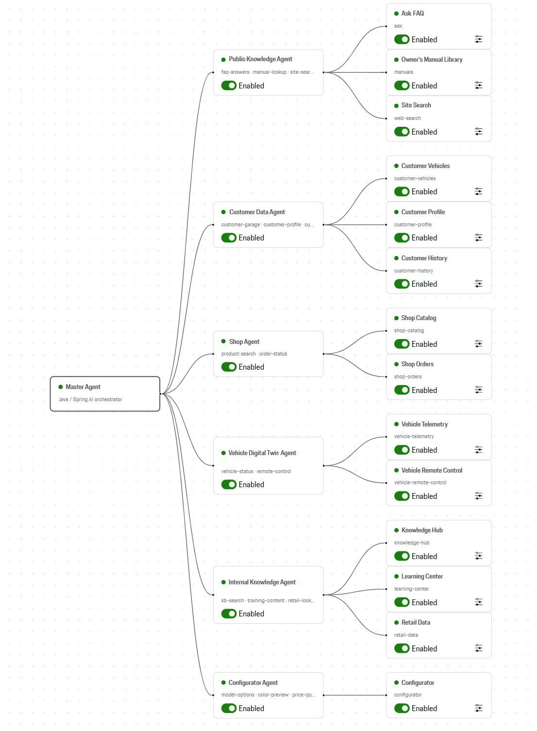
The interface uses the Porsche Design System, so for the purposes of the demo I call it the Porsche Assistant. All data sources aremocked and no Porsche data was used. The demo is an architecture demonstrator, not a production product.

Consider the question: “How do I change the battery in my car’s remote control?”

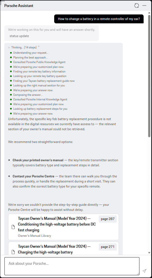
Please note important elements of the screenshot. The assistant has done a lot of work to understand the question, plan how to solve my issue, collect data from my profile, discover what car I have, look for the manual for it, and even cross-check the answer against an internal knowledge base. The panel labeled “Thinking” in the screenshot is better understood as an execution-progress view: it shows observable system activity, not the model’s private chain of thought. The answer is not very useful due to generated in-place tool responses in my demo, but some mocked resources are still returned to address my question.

The flow is better visible in Langfuse as an animation of all components running.

Because the first-choice agent returned a weak, unsatisfactory answer, the system slowed down a little – but that is exactly what shows it can recover from poor agent responses at the cost of time, and it puts the reasoning-based circuit breaker on display, calling off the hunt for the perfect answer once it is clear there isn’t one.

The demo proves that both MCP and A2A can transfer rich responses and that with a well-designed entry point, you can implement a “thinking” process built on your own data and your own capabilities. You can not only connect data sources but also execute actions, e.g., schedule a service appointment, order a gadget from the company shop, configure a new car, or unlock your own car through the same API the mobile app uses.

Further steps: Evaluation and load testing

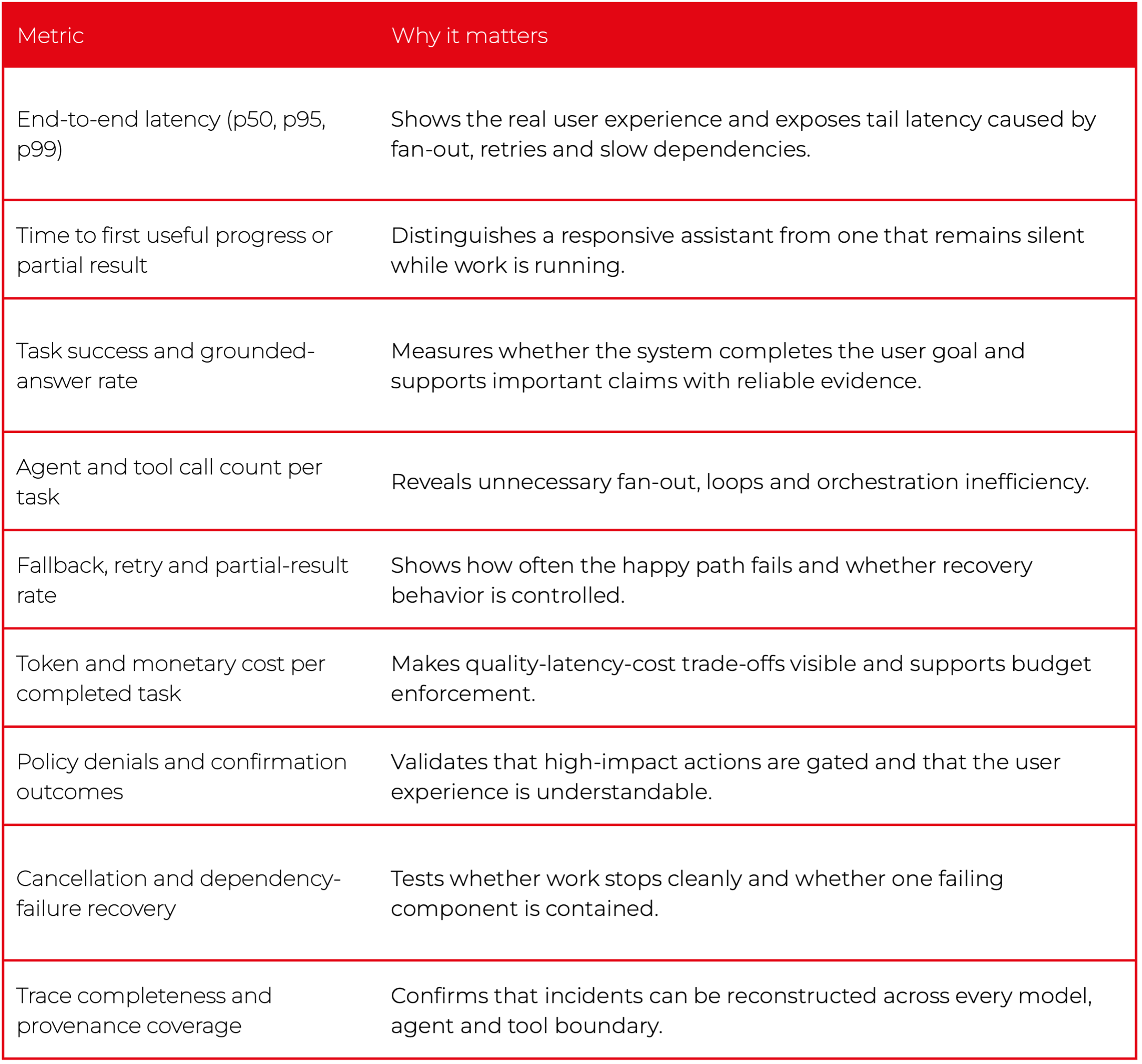
A convincing demo should be followed by a small evaluation and load-testing program. At minimum, I would track the following metrics:

Conclusion: AI assistant architecture in 2026

The answer to “How do you turn a chatbot into an AI assistant?” becomes standardized and protocolized, but production quality still comes from the boundaries and controls around those protocols. Use A2A for genuinely independent agents. Keep deterministic policy outside the LLM. Define shared data contracts. Bound the execution graph. Propagate traces. Require confirmation before high-impact actions. Measure latency, quality, cost and failure recovery.

Do that, and flexibility becomes controlled extensibility rather than agentic spaghetti. That, to me, is what AI-assistant architecture means in 2026.

FAQ

‍
What is the difference between MCP and A2A?

MCP standardizes tool calling: you point the model at an MCP server's URL and the SDK provides context and executes tools. A2A standardizes how one agent calls another — with discovery, long polling, asynchronous responses, authorization, input requests and streaming. Use A2A when the remote component is an autonomous system that reasons, plans and maintains state; use MCP to expose tools and data.

How do you turn a chatbot into an AI assistant in 2026?

With MCP and A2A, used wisely. The proposal is a three-layer, tree-like structure: one or more entry-point (master) agents that call working agents, which in turn call MCP servers with tools — processed asynchronously, with circuit breakers, shared data contracts and end-to-end tracing.

What is the Model Context Protocol (MCP)?

MCP is a way to provide context to the model. It unifies tool calling and automates system-prompt provisioning: you provide the MCP server's URL and the SDK calls tools under the hood, while the server maintainer takes care of tool descriptions and updates.

What is the Agent-to-Agent (A2A) protocol?

A2A is a standardized way for one agent to call another — complete with agent discovery, long polling, asynchronous responses, authorization, input requests and streaming. It is a good fit when the remote component is autonomous and owned and deployed independently.

Why replace the SDK-based MCP integration with custom code or a proxy?

The SDK runs the whole request-response loop automatically, which limits monitoring, prevents you from stopping hallucinated calls or attaching metadata such as PII, and forces the LLM to process extra fields. Custom code or an MCP proxy lets you use structuredContent, enrich requests with authorization or metadata, and forward extra fields to the master agent.

How do you handle access control (RBAC) for MCP tools?

Add a custom header to MCP calls and verify user permissions at two points — when listing tools and when executing them. OAuth 2.0 Token Exchange with token caching is recommended; passing tokens through as-is is discouraged and in fact forbidden by MCP.

How do you monitor a multi-agent AI assistant?

Give each component its own Langfuse integration and report observations against the parent by passing the parent observation ID as request metadata, keeping server clocks synchronized. Newer MCP versions also document traceparent, tracestate and baggage propagation so a tool call can appear in a single OpenTelemetry-compatible trace.

‍

Do you have an application in the AWS cloud? Do you have several microservices you would like to monitor? Or maybe you’re starting your new project and looking for some good-looking, well-designed infrastructure? Look no further - you are in the right place!

We’ve spent some time building and managing microservices and cloud-native infrastructure so we provide you with a guide covering the main challenges and proven solutions.

In this series, we describe the following topics:

1. How to create a well-designed architecture with microservices and a cloud-config server?
2. How to collect metrics and logs in a common dashboard?
3. How to secure the entire stack?

Monitoring your microservices - assumptions

Choosing Grafana for such a project seems obvious, as the tool is powerful, fast, user-friendly, customizable, and easy to maintain. Grafana works perfectly with Prometheus and Loki. Prometheus is a metric sink that collects metrics from multiple sources and sends them to the target monitoring system. Loki does the very same operation for logs. Both collectors are designed to be integrated with Grafana.

See the diagram below to better understand our architecture:

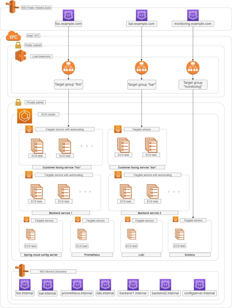
Let’s analyze the diagram for a moment. On the top, there is a publicly visible hosted zone in Route 53, the DNS “entry” to our system, with 3 records: two application services available over the internet and an additional monitoring service for our internal purposes.

Below, there is a main VPC with two subnets: public and private. In the public one, we have load balancers only, and in the private one, there is an ECS cluster. In the cluster, we have few services running using Fargate: two with internet-available APIs, two for internal purposes, one Spring Cloud Config Server, and our monitoring stack: Loki, Prometheus, and Grafana. At the bottom of the diagram, you can also find a Service Discovery service (AWS CloudMap) that creates entries in Route 53, to enable communication inside our private subnet.

Of course, for readability reasons, we omit VPC configuration, services dependencies (RDS, Dynamo, etc.), CI/CD, and all other services around the core. You can follow this guide covering building AWS infrastructure.

To sum up our assumptions:

• We use an infra-as-a-code approach with Terraform
• There are few Internet-facing services and few for internal purposes in our private subnet
• Internet-facing services are exposed via load balancers in the public subnet
• We use the Fargate launch type for ECS tasks
• Some services can be scaled with ECS auto-scaling groups
• We use Service Discovery to redeploy and scale without manual change of IP’s, URL’s or target groups
• We don’t want to repeat ourselves so we use a Spring Cloud Config Server as a main source of configuration
• We use Grafana to see synchronized metrics and logs
• (what you cannot see on the diagram) We use encrypted communication everywhere - including communication between services in a private subnet

Basic AWS resources

In this article, we assume you have all basic resources already created and correctly configured: VPC, subnets, general security groups, network ACLs, network interfaces, etc. Therefore we’re going to focus on resources visible on the diagram above, crucial from a monitoring point of view.

Let’s create the first common resource:

resource "aws_service_discovery_private_dns_namespace" "namespace_for_environment" {

name = "internal"

vpc = var.vpc_id

}

This is the Service Discovery visible in the lower part of the diagram. We’re going to fill it in a moment.

By the way, above, you can see an example, how we’re going to present listings. You will need to adjust some variables for your needs (like var .vpc_id ). We strongly recommend using Terragrunt to manage dependencies between your Terraform modules, but it’s out of the scope of this paper.

Your services without monitoring

Internet-facing services

Now let’s start with the first application. We need something to monitor.

resource "aws_route53_record" "foo_entrypoint" {

zone_id = var.zone_environment_id

name = "foo"

type = "A"

set_identifier = "foo.example.com"



alias {

name = aws_lb.foo_ecs_alb.dns_name

zone_id = aws_lb.foo_ecs_alb.zone_id

evaluate_target_health = true

}



latency_routing_policy {

region = var.default_region

}

}

This is an entry for Route53 to access the internet-facing “foo” service. We’ll use it to validate a TLS certificate later.

resource "aws_lb" "foo_ecs_alb" {

name = "foo"

internal = false

load_balancer_type = "application"

security_groups = [

aws_security_group.alb_sg.id

]

subnets = var.vpc_public_subnet_ids

}



resource "aws_lb_target_group" "foo_target_group" {

name = "foo"

port = 8080

protocol = "HTTP"

target_type = "ip"

vpc_id = var.vpc_id



health_check {

port = 8080

protocol = "HTTP"

path = "/actuator/health"

matcher = "200"

}

depends_on = [

aws_lb.foo_ecs_alb

]

}



resource "aws_lb_listener" "foo_http_listener" {

load_balancer_arn = aws_lb.foo_ecs_alb.arn

port = "8080"

protocol = "HTTP"



default_action {

type = "forward"

target_group_arn = aws_lb_target_group.foo_target_group.arn

}

}



resource "aws_security_group" "alb_sg" {

name = "alb-sg"

description = "Inet to ALB"

vpc_id = var.vpc_id



ingress {

protocol = "tcp"

from_port = 8080

to_port = 8080

cidr_blocks = [

"0.0.0.0/0"

]

}



egress {

protocol = "-1"

from_port = 0

to_port = 0

cidr_blocks = [

"0.0.0.0/0"

]

}

}

OK, what do we have so far?

Besides the R53 entry, we’ve just created a load balancer, accepting traffic on 8080 port and transferring it to the target group called foo_target_group . We use a default Spring Boot " /actuator/health " health check endpoint (you need to have spring-boot-starter-actuator dependency in your pom) and a security group allowing ingress traffic to reach the load balancer and all egress traffic from the load balancer.

Now, let’s create the service.

resource "aws_ecr_repository" "foo_repository" {

name = "foo"

}



resource "aws_ecs_task_definition" "foo_ecs_task_definition" {

family = "foo"

network_mode = "awsvpc"

requires_compatibilities = ["FARGATE"]

cpu = "512"

memory = "1024"

execution_role_arn = var.ecs_execution_role_arn



container_definitions = <<TASK_DEFINITION

[

{

"cpu": 512,

"image": "${aws_ecr_repository.foo_repository.repository_url}:latest",

"memory": 1024,

"memoryReservation" : 512,

"name": "foo",

"networkMode": "awsvpc",

"essential": true,

"environment" : [

{ "name" : "SPRING_CLOUD_CONFIG_SERVER_URL", "value" : "configserver.internal" },

{ "name" : "APPLICATION_NAME", "value" : "foo" }

],

"portMappings": [

{

"containerPort": 8080,

"hostPort": 8080

}

]

}

]

TASK_DEFINITION

}



resource "aws_ecs_service" "foo_service" {

name = "foo"

cluster = var.ecs_cluster_id

task_definition = aws_ecs_task_definition.foo_ecs_task_definition.arn

desired_count = 2

launch_type = "FARGATE"



network_configuration {

subnets = var.vpc_private_subnet_ids

security_groups = [

aws_security_group.foo_lb_to_ecs.id,

aws_security_group.ecs_ecr_security_group.id,

aws_security_group.private_security_group.id

]

}

service_registries {

registry_arn = aws_service_discovery_service.foo_discovery_service.arn

}



load_balancer {

target_group_arn = aws_lb_target_group.foo_target_group.arn

container_name = "foo"

container_port = 8080

}



depends_on = [aws_lb.foo_ecs_alb]

}

You can find just three resources above, but a lot of configuration. The first one is easy - just an ECR for the image of your application. Then we have a task definition. Please pay attention to environment variables SPRING_CLOUD_CONFIG_SERVER_URL - this is an address of our config server inside our internal Service Discovery domain. The third one is an ECS service.

As you can see, it uses some magic of ECS Fargate - automatically registering new tasks in a Service Discovery ( service_registries section) and a load balancer ( load_balancer section). We just need to wait until the load balancer is created ( depends_on = [aws_lb.foo_ecs_alb] ). If you want to add some autoscaling, this is the right place to put it in. You’re also ready to push your application to the ECR if you already have one. We’re going to cover the application's important content later in this article. The ecs_execution_role_arn is just a standard role with AmazonECSTaskExecutionRolePolicy , allowed to be assumed by ECS and ecs-tasks.

Let’s discuss security groups now.

resource "aws_security_group" "foo_lb_to_ecs" {

name = "allow_lb_inbound_foo"

description = "Allow inbound Load Balancer calls"

vpc_id = var.vpc_id



ingress {

from_port = 8080

protocol = "tcp"

to_port = 8080

security_groups = [aws_security_group.foo_alb_sg.id]

}

}



resource "aws_security_group" "ecs_to_ecr" {

name = "allow_ecr_outbound"

description = "Allow outbound traffic for ECS task, to ECR/docker hub"

vpc_id = aws_vpc.main.id



egress {

from_port = 443

to_port = 443

protocol = "tcp"

cidr_blocks = ["0.0.0.0/0"]

}



egress {

from_port = 53

to_port = 53

protocol = "udp"

cidr_blocks = ["0.0.0.0/0"]

}



egress {

from_port = 53

to_port = 53

protocol = "tcp"

cidr_blocks = ["0.0.0.0/0"]

}

}



resource "aws_security_group" "private_inbound" {

name = "allow_inbound_within_sg"

description = "Allow inbound traffic inside this SG"

vpc_id = var.vpc_id



ingress {

from_port = 0

to_port = 0

protocol = "-1"

self = true

}



egress {

from_port = 0

to_port = 0

protocol = "-1"

self = true

}

}

As you can see, we use three groups - all needed. The first one allows the load balancer located in the public subnet to call the task inside the private subnet. The second one allows our ECS task to poll its image from the ECR. The last one allows our services inside the private subnet to talk to each other - such communication is allowed by default, only if you don’t attach any specific group (like the load balancer’s one), therefore we need to explicitly permit this communication.

There is just one piece needed to finish the “foo” service infrastructure - the service discovery service entry.

resource "aws_service_discovery_service" "foo_discovery_service" {

name = "foo"

description = "Discovery service name for foo"



dns_config {

namespace_id = aws_service_discovery_private_dns_namespace.namespace_for_environment.id



dns_records {

ttl = 100

type = "A"

}

}

}

It creates a “foo” record in an “internal” zone. So little and yet so much. The important thing here is - this is a multivalue record, which means it can cover 1+ entries - it provides basic, equal-weight autoscaling during normal operation but Prometheus can dig out from such a record each IP address separately to monitor all instances.

Now some good news - you can simply copy-paste the code of all resources with names prefixed with “foo_” and create “bar_” clones for the second, internet-facing service in the project. This is what we love Terraform for.

Backend services (private subnet)

This part is almost the same as the previous one, but we can simplify some elements.

resource "aws_ecr_repository" "backend_1_repository" {

name = "backend_1"

}



resource "aws_ecs_task_definition" "backend_1_ecs_task_definition" {

family = "backend_1"

network_mode = "awsvpc"

requires_compatibilities = ["FARGATE"]

cpu = "512"

memory = "1024"

execution_role_arn = var.ecs_execution_role_arn



container_definitions = <<TASK_DEFINITION

[

{

"cpu": 512,

"image": "${aws_ecr_repository.backend_1_repository.repository_url}:latest",

"memory": 1024,

"memoryReservation" : 512,

"name": "backend_1",

"networkMode": "awsvpc",

"essential": true,

"environment" : [

{ "name" : "_JAVA_OPTIONS", "value" : "-Xmx1024m -Xms512m" },

{ "name" : "SPRING_CLOUD_CONFIG_SERVER_URL", "value" : "configserver.internal" },

{ "name" : "APPLICATION_NAME", "value" : "backend_1" }

],

"portMappings": [

{

"containerPort": 8080,

"hostPort": 8080

}

]

}

]

TASK_DEFINITION

}



resource "aws_ecs_service" "backend_1_service" {

name = "backend_1"

cluster = var.ecs_cluster_id

task_definition = aws_ecs_task_definition.backend_1_ecs_task_definition.arn

desired_count = 1

launch_type = "FARGATE"



network_configuration {

subnets = var.vpc_private_subnet_ids

security_groups = [

aws_security_group.ecs_ecr_security_group.id,

aws_security_group.private_security_group.id

]

}



service_registries {

registry_arn = aws_service_discovery_service.backend_1_discovery_service.arn

}

}



resource "aws_service_discovery_service" "backend_1_discovery_service" {

name = "backend1"

description = "Discovery service name for backend 1"



dns_config {

namespace_id = aws_service_discovery_private_dns_namespace.namespace_for_environment.id



dns_records {

ttl = 100

type = "A"

}

}

}

As you can see, all resources related to the load balancer are gone. Now, you can copy the code about creating the backend_2 service.

So far, so good. We have created 4 services, but none will start without the config server yet.

Config server

The infrastructure for the config server is similar to the backed services described above. It simply needs to know all other services’ URLs. In the real-world scenario, the configuration may be stored in a git repository or in the DB, but it’s not needed for this article, so we’ve used a native config provider, with all config files stored locally.

We would like to dive into some code here, but there is not much in this module yet. To make it just working, we only need this piece of code:

@SpringBootApplication

@EnableConfigServer

public class CloudConfigServer {

public static void main(String[] arguments) {

run(CloudConfigServer.class, arguments);

}

}

and few dependencies.

<dependency>

<groupId>org.springframework.cloud</groupId>

<artifactId>spring-cloud-config-server</artifactId>

</dependency>

<dependency>

<groupId>org.springframework.boot</groupId>

<artifactId>spring-boot-starter-security</artifactId>

</dependency>

<dependency>

<groupId>org.springframework.boot</groupId>

<artifactId>spring-boot-starter-web</artifactId>

</dependency>

We also need some extra config in the pom.xml file.

<parent>

<groupId>org.springframework.boot</groupId>

<artifactId>spring-boot-starter-parent</artifactId>

<version>2.4.2</version>

</parent>



<dependencyManagement>

<dependencies>

<dependency>

<groupId>org.springframework.cloud</groupId>

<artifactId>spring-cloud-dependencies</artifactId>

<version>2020.0.1</version>

<type>pom</type>

<scope>import</scope>

</dependency>

</dependencies>

</dependencyManagement>



<build>

<plugins>

<plugin>

<groupId>org.springframework.boot</groupId>

<artifactId>spring-boot-maven-plugin</artifactId>

</plugin>

</plugins>

</build>

That’s basically it - you have your own config server. Now, let’s put some config inside. The Structure of the server is as follows.

config_server/

├─ src/

│ ├─ main/

│ ├─ java/

│ ├─ com/

│ ├─ example/

│ ├─ CloudConfigServer.java

│ ├─ resources/

│ ├─ application.yml (1)

│ ├─ configforclients/

│ ├─ application.yml (2)

As there are two files called application.yml we’ve added numbers (1), (2) at the end of lines to distinguish them. So the application.yml (1) file is there to configure the config server itself. Its content is as follows:

server:

port: 8888

spring:

application:

name: spring-cloud-config-server

profiles:

include: native

cloud:

config:

server:

native:

searchLocations: classpath:/configforclients

management:

endpoints:

web:

exposure:

include: health

With the “native” configuration, the entire classpath:/ and classpath:/config are taken as a configuration for remote clients. Therefore, we need this line:
spring.cloud.config.server.native.searchLocations: classpath:/configforclients to distinguish the configuration for the config server itself and for the clients. The client’s configuration is as follows:

address:

foo: ${FOO_URL:http://localhost:8080}

bar: ${BAR_URL:http://localhost:8081}

backend:

one: ${BACKEND_1_URL:http://localhost:8082}

two: ${BACKEND_2_URL:http://localhost:8083}

management:

endpoints:

web:

exposure:

include:health

spring:

jackson:

default-property-inclusion: non_empty

time-zone: Europe/Berlin

As you can see, all service discovery addresses are here, so they can be used by all clients. We also have some common configurations, like Jackson-related, and one important for the infra - to expose health checks for load balancers.

If you use Spring Boot Security (I hope you do), you can disable it here - it will make accessing the config server simpler, and, as it’s located in the private network and we’re going to encrypt all endpoints in a moment - you don’t need it. Here is an additional file to disable it.

@Configuration

@EnableWebSecurity

public class WebSecurityConfig extends WebSecurityConfigurerAdapter {



@Override

public void configure(WebSecurity web) throws Exception {

web.ignoring().antMatchers("/**");

getHttp().csrf().disable();

}

}

Yes, we know, it's strange to use @EnableWebSecurity to disable web security, but it’s how it works. Now, let’s configure clients to read those configurations.

Config clients

First of all, we need two dependencies.

<dependency>

<groupId>org.springframework.cloud</groupId>

<artifactId>spring-cloud-starter-bootstrap</artifactId>

</dependency>

<dependency>

<groupId>org.springframework.cloud</groupId>

<artifactId>spring-cloud-starter-config</artifactId>

</dependency>

We assume you have all Spring-Boot related dependencies already in place.

As you can see, we need to use bootstrap, so instead of the application.yml file, we’re going to use bootstrap.yml(which is responsible for loading configuration from external sources):

main:

banner-mode: 'off'

cloud:

config:

uri: ${SPRING_CLOUD_CONFIG_SERVER:http://localhost:8888}

There are only two elements here. We use the first one just to show you that some parameters simply cannot be set using the config server. In this example, main.banner-mode is being read before accessing the config server, so if you want to disable the banner (or change it) - you need to do it in each application separately. The second property - cloud.config.uri - is obviously a pointer to the config server. As you can see, we use a fallback value to be able to run everything both in AWS and local machines.

Now, with this configuration, you can really start every service and make sure that everything works as expected.

Monitoring your microservices - conclusion

That was the easy part. Now you have a working application, exposed and configurable. We hope you can tweak and adjust it for your own needs. In the next part we’ll dive into a monitoring topic.

Have you ever wanted to build your own Android? It’s easy according to the official manual, but it’s getting harder on a Windows (or Mac) machine, or if you’d like to run it on physical hardware. Still too easy? Let’s build Android Automotive OS – the same source code, but another layer of complexity. In this manual, we’ll cover all steps needed to build and run Android Automotive OS 11 AOSP on Raspberry Pi 4B using Windows. The solution is not perfect, however. The most principal issue is a lack of Google Services because the entire AAOS is on an open-source project and Google doesn’t provide its services this way. Nevertheless, let’s build the open-source version first, and then we can try to face incoming issues.

TL;DR: If you don't want to configure and build the system step-by-step, follow the simplified instruction at  https://github.com/grapeup/aaos_11_local_manifest

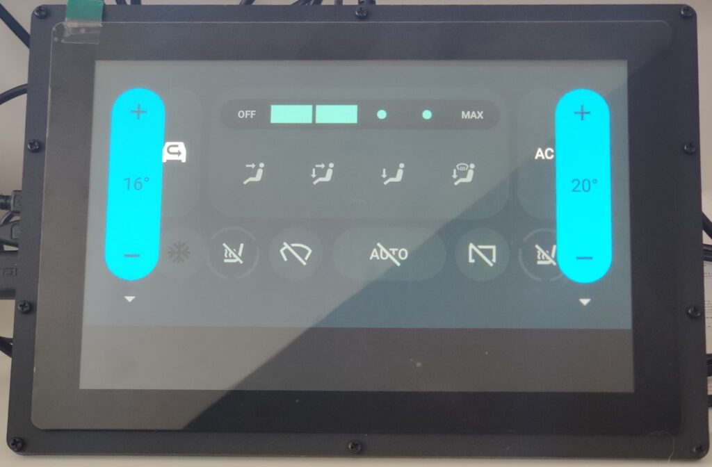
Prerequisites

Hardware

If you want to run the system on a physical device, you need one. I use the Raspberry Pi 4 model B with 8GB of RAM (  https://www.raspberrypi.com/products/raspberry-pi-4-model-b/ ). By the way, if you want to build and run an emulator from the source, it’s also possible, but there is a small limitation – packaging the emulator to a zip file, moving it to another computer, or even running it under Android Studio was introduced in Android 12.

To power your Raspberry, you need a power adapter (USB C, min. 5V 3A). I use the Raspberry-official 5.1V 3A model. You can also power the Raspberry computer from your desktop/laptop’s USB port, especially if you’re going to debug it via a serial connection. Check the “If it doesn’t work” section below for the required hardware.

Another piece of hardware needed is an SD card. In theory, 4GB is all you need, however, I recommend buying a larger card to have some extra space for  your applications on Android . I use 32GB and 64GB cards. You’ll also need a built-in or external card reader. I use the latter.

The next step is a screen. It’s optional but fancy. You can connect your mouse and optionally keyboard to your Raspberry Pi via USB and connect any display you have via micro-HDMI but using a touch screen is much more intuitive. I use a Waveshare 10-inch screen dedicated to Raspberry (  https://www.waveshare.com/wiki/10.1inch_HDMI_LCD_(B)_(with_case ). The screen box has a place to screw the Raspberry too, so you don’t need any extra case. You can also buy it with a power adapter and a display cable.

If you don’t buy a bundle, make sure you have all necessary accessories: micro-HDMI – HDMI cable to connect a screen (Waveshare or any other), USB A – USB mini A cable to connect a touch sensor of the screen, USB mini A 5V 3A adapter to power the screen.

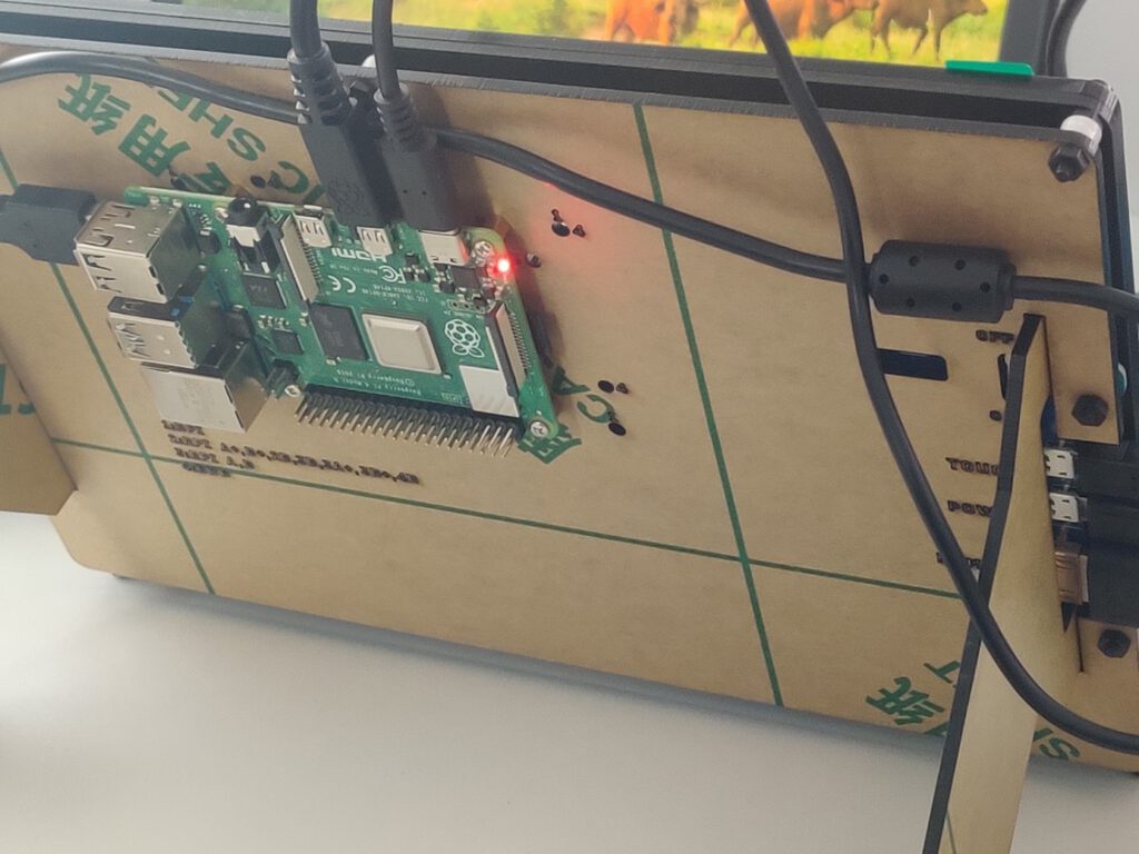
Of course, you need a computer. In this manual, we use a Windows machine with at least 512GB of storage (the Android source is huge) and 16GB of RAM.

Software

You can probably build everything in pure Windows, but the recommended method is to use WSL. I assume you already have it installed, so just make sure you have the newest WSL2 version. If you have never used WSL before, see the full manual here  https://learn.microsoft.com/en-us/windows/wsl/install .

 WSL adjustments

The standard WSL installation uses a too-small virtual drive and limited RAM, so you need to adjust it.

Let’s start with the disk. Make sure the WSL is shut down by running ‘wsl –shutdown’ in the command prompt. Open Windows Command Prompt with admin privileges and enter ‘diskpart  ’. Then run ‘select vdisk file=”<path to WSL drive file>”’. For me, the path is “C:\Users\<user>\AppData\Local\Packages\CanonicalGroupLimited.Ubuntu_<WSL_instance_id>\LocalState\ext4.vhdx  ”. Now you can expand it with the command ‘expand vdisk maximum=512000’. Around 300GB is enough for Android 11, but if you want to play with multiple branches of Android at the same time, you need more space. Now you can close the diskpart with the ‘exit’ command. Next, open the WSL and run ‘sudo resize2fs /dev/sdb 512000M’. I assume you have only a single drive attached to the WSL and it’s visible in the Linux subsystem as /dev/sdb. You can check it with the commands ‘sudo mount -t devtmpfs none /dev || mount | grep ext4’.

Now, let’s adjust the memory. Stop the WSL again. Open your home directory in Windows and open .wslconfig file. Create it if this file doesn’t exist yet. In the file, you need to create a [wsl2] section and memory configuration. The complete file should look like this:

[wsl2]
memory=16GB

As you can see, I’ve attached 16GB to the virtual machine. It’s assigned dynamically, according to needs, but you must be aware that the virtual machine can take all of it, so if you allow it to eat your entire RAM, it can force your Windows to use a hard disk to survive (which will slow everything down significantly).

 Disclaimer:

 Building Android on 8 cores, 16GB RAM machine takes around 4 hours. If you want to do it faster or you don’t have a computer powerful enough at your home or office, you can consider building in the cloud. Simple AWS EC2 with 32 cores and 64GB of memory does the job in one hour (to download and build) and costs just a few bucks.

Let's get ready to rumble!!!

..or at least to building.

More prerequisites

We need some software but not much. Just install the following packages. This set of libraries allows you to build Android Automotive OS versions 11 to 13.

sudo apt update && sudo apt install gcc-aarch64-linux-gnu libssl-dev bc python3-setuptools repo python-is-python3 libncurses5 zip unzip make gcc flex bison -y

Source code downloading

Let’s create a home directory for our android and download sources.

mkdir android-11.0.0_r48 && cd android-11.0.0_r48
repo init -u https://android.googlesource.com/platform/manifest -b android-11.0.0_r48 --partial-clone --clone-filter=blob:limit=10M
git clone https://github.com/android-rpi/local_manifests .repo/local_manifests -b arpi-11
repo sync

“repo init” will ask you for some personal data. It’s collected by Google. To learn more about optimizations here, check this manual:  https://docs.gitlab.com/ee/topics/git/partial_clone.html . ‘git clone’ adds a custom code from Android RPI project (  https://groups.google.com/g/android-rpi ) with drivers for your Raspberry Pi. The project is great and it’s all you need if you want to run Android TV. To run Android Automotive OS, we’ll need to adjust it slightly (see “Adjustments” section below). ‘repo sync’ will take some time because you need to download around 200GB of code. If you have a powerful machine with a great Internet connection, you can use more threads with ‘-j X’ parameter added to the command. The default thread count is 4. If you have already synchronized your source code without android-rpi local manifest, you need to add --force-sync to the ’repo-sync’ command.

Adjustments

 All changes from this section can download as a patch file attached to this article. See the “Path file” section below.

Android-rpi provides Android TV for Raspberry Pi. We need to remove the TV-related configuration and add the Automotive OS one.

Let’s start with removing unnecessary files. You can safely remove the following files and directories:

•  device/arpi/rpi4/overlay/frameworks/base/core/res/res/anim
•  device/arpi/rpi4/overlay/frameworks/base/core/res/res/values-television
•  device/arpi/rpi4/overlay/frameworks/base/core/res/res/values/dimens.xml
•  device/arpi/rpi4/overlay/frameworks/base/core/res/res/values/styles.xml
•  device/arpi/rpi4/overlay/frameworks/base/packages

To remove the user notice screen not needed in Automotive OS, create a new file device/arpi/rpi4/overlay/packages/services/Car/service/res/values/config.xml with the following content:

<?xml version="1.0" encoding="utf-8"?>
<resources xmlns:xliff="urn:oasis:names:tc:xliff:document:1.2">
<string name="config_userNoticeUiService" translatable="false"></string>
</resources>

To replace the basic TV overlay config with the Automotive overlay config, adjust the configuration in device/arpi/rpi4/overlay/frameworks/base/core/res/res/values/config.xml.

Remove:

•  <integer name="config_defaultUiModeType">4</integer> <!--disable forced UI_MODE_TYPE_TELEVISION, as there is only MODE_TYPE_CAR available now-->
•  <integer name="config_longPressOnHomeBehavior">0</integer> <!--disable home button long press action-->
•  <bool name="config_hasPermanentDpad">true</bool> <!--disable D-pad-->
•  <string name="config_appsAuthorizedForSharedAccounts">;com.android.tv.settings;</string> <!--remove unnecessary access for a shared account as there is nothing in com.android.tv.* now-->

… and add:

•  <bool name="config_showNavigationBar">true</bool> <!--enable software navigation bar, as there is no hardwave one-->
•  <bool name="config_enableMultiUserUI">true</bool> <!--enable multi-user, as AAOS uses background processes called in another sessions -->
•  <integer name="config_multiuserMaximumUsers">8</integer> <!--set maximum user count, required by the previous one-->

Now let’s rename the android-rpi original /device/arpi/rpi4/rpi4.mk to /device/arpi/rpi4/android_rpi4.mk. We need to adjust the file a little bit.

Remove the following variables definitions. Some of them you will re-create in another file, while some of them are not needed.

•  PRODUCT_NAME
•  PRODUCT_DEVICE
•  PRODUCT_BRAND
•  PRODUCT_MANUFACTURER
•  PRODUCT_MODEL
•  USE_OEM_TV_APP
•  DEVICE_PACKAGE_OVERLAYS
•  PRODUCT_AAPT_PRED_CONFIG
•  PRODUCT_CHARACTERISTICS

Remove the following invocations. We’re going to call necessary external files in another mk file.

•  $(call inherit-product, device/google/atv/products/atv_base.mk)
•  $(call inherit-product, $(SRC_TARGET_DIR)/product/core_64_bit_only.mk)
•  $(call inherit-product, $(SRC_TARGET_DIR)/product/languages_full.mk)
•  include frameworks/native/build/tablet-10in-xhdpi-2048-dalvik-heap.mk

In PRODUCT_PROPERTY_OVERRIDES remove debug.drm.mode.force=1280x720 and add the following properties. This way you remove the TV launcher configuration and override the default automotive launcher configuration.

•  dalvik.vm.dex2oat64.enabled=true
•  keyguard.no_require_sim=true
•  ro.logd.size=1m

Now you need to completely remove the android-rpi TV launcher and add RenderScript support for Automotive OS. In PRODUCT_PACKAGES remove:

•  DeskClock
•  RpLauncher

… and add:

•  librs_jni

Create a new rpi4.mk4 with the following content:

PRODUCT_PACKAGE_OVERLAYS += device/generic/car/common/overlay
$(call inherit-product, $(SRC_TARGET_DIR)/product/core_64_bit.mk)
$(call inherit-product, device/arpi/rpi4/android_rpi4.mk)
$(call inherit-product, $(SRC_TARGET_DIR)/product/full_base.mk)
$(call inherit-product, device/generic/car/common/car.mk)
PRODUCT_SYSTEM_DEFAULT_PROPERTIES += \
   android.car.number_pre_created_users=1 \
   android.car.number_pre_created_guests=1 \
   android.car.user_hal_enabled=true
DEVICE_PACKAGE_OVERLAYS += device/arpi/rpi4/overlay device/generic/car/car_x86_64/overlay

PRODUCT_NAME := rpi4
PRODUCT_DEVICE := rpi4
PRODUCT_BRAND := arpi
PRODUCT_MODEL := Raspberry Pi 4
PRODUCT_MANUFACTURER := GrapeUp and ARPi

Due to the license, remember to add yourself to the PRODUCT_MANUFACTURER field.

Now you have two mk files – android-rpi.mk is borrowed from android-rpi project and adjusted, and rpi.mk contains all changes for Automotive OS. You can meld these two together or split them into more files if you’d like, but keep in mind that the order of invocations does matter (not always, but still).

As Android Automotive OS is bigger than Android TV, we need to increase the system partition size to fit the new image. In device/arpi/rpi4/BoardConfig.mk increase BOARD_SYSTEMIMAGE_PARTITION_SIZE to 2147483648, which means 2GB.

You need to apply all changes described in  https://github.com/android-rpi/device_arpi_rpi4/wiki/arpi-11-:-framework-patch too. Those changes are also included in the  patch file attached .

If you use the 8GB version of Raspberry Pi, you need to replace device/arpi/rpi4/boot/fixup4.dat and device/arpi/rpi4/boot/start4.elf files. You can find the correct files in the patch file attached or you may use the official source:  https://github.com/raspberrypi/firmware/tree/master/boot . It’s probably not needed for 4GB version of Raspberry, but I don’t have such a device for verification.

Path file

If you prefer to apply all changes described above as a single file, go to your sources directory and run ‘git apply --no-index <path_to_patch_file>  ’. There is also a boot animation replaced in the  patch file . If you want to create one of your own, follow the official manual here:  https://android.googlesource.com/platform/frameworks/base/+/master/cmds/bootanimation/FORMAT.md .

Now we can build!

That’s the easy part. Just run a few commands from below. Firstly, we need to build a custom kernel for Android. ‘merge_config.sh’ script just configures all variables required. The first ‘make’ command builds the real kernel image (which can take a few minutes). Next, build a device tree configuration.

cd kernel/arpi
ARCH=arm64 scripts/kconfig/merge_config.sh arch/arm64/configs/bcm2711_defconfig kernel/configs/android-base.config kernel/configs/android-recommended.config
ARCH=arm64 CROSS_COMPILE=aarch64-linux-gnu- make Image.gz
ARCH=arm64 CROSS_COMPILE=aarch64-linux-gnu- DTC_FLAGS="-@" make broadcom/bcm2711-rpi-4-b.dtb
ARCH=arm64 CROSS_COMPILE=aarch64-linux-gnu- DTC_FLAGS="-@" make overlays/vc4-kms-v3d-pi4.dtbo
cd ../..

The next part is to build the entire system. “envsetup.sh” script sets up variables and adds custom commands to your terminal. Then you can pick the correct pair of Android versions and devices with “lunch”. You can run it without parameters to see (almost) all possible configurations. In this step, you can decide to build a system for dedicated hardware (eg. Dragonboard) and switch between phone/tablet/TV/wearable/automotive versions of Android. The last line is a real building. We can’t run just “make” or “m”, as documented in the official manual because we need to create three specific images to write them on an SD card and run them on Raspberry Pi. Replace “X” in ‘-j X’ with the number of threads you want to use. The default value is the number of logical processors on your computer.

source build/envsetup.sh
lunch rpi4-eng
make -j X ramdisk systemimage vendorimage

I hope you have a delightful book next to you because the last building takes a few hours depending on your hardware. Good news!  If you need to adapt something and build again, in most cases you just need the three last lines (or even just the very last one) – to source the environment setup, to pick the lunch configuration, and to make ramdisk, system, and vendor images. And it takes hours for the first time only.

Creating an SD card

This step seems to be easy, but it isn’t. WSL doesn’t contain drivers for the USB card reader. You can use usbip to forward a device from Windows to the subsystem, but it doesn’t work well with external storage without partitions. The solution is a VirtualBox with Ubuntu installed. Just create a virtual machine, install Ubuntu, and install Guest Additions. Then you can connect the card reader and pass it to the virtual machine. If you’re a minimalist, you can use Ubuntu Server or any other Linux distribution you like. Be aware that using a card reader built into your computer may be challenging depending on drivers and the hardware connection type (USB-like, or PCI-e).

Now, you need to create a partition schema on the SD card. I assume the card is loaded to the system as /dev/sdb. Check your configuration before continuing to avoid formatting your main drive or another disaster. Let’s erase the current partition table and create a new one.

sudo umount /dev/sdb*
sudo wipefs -a /dev/sdb
sudo fdisk /dev/sdb

Now let’s create partitions. First, you need a 128MB active partition of the W95 FAT32 (LBA) type, second a 2GB Linux partition, third a 128MB Linux partition, and the rest of the card for user data (also Linux partition). Here’s how to navigate through fdisk menu to configure all partitions.

Welcome to fdisk (util-linux 2.37.2).
Changes will remain in memory only, until you decide to write them.
Be careful before using the write command.
Device does not contain a recognized partition table.
Created a new DOS disklabel with disk identifier 0x179fb9bc.
Command (m for help): n
Partition type
  p   primary (0 primary, 0 extended, 4 free)
  e   extended (container for logical partitions)
Select (default p):
Using default response p.
Partition number (1-4, default 1):
First sector (2048-61022207, default 2048):
Last sector, +/-sectors or +/-size{K,M,G,T,P} (2048-61022207, default 61022207): +128M
Created a new partition 1 of type 'Linux' and of size 128 MiB.
Command (m for help): a
Selected partition 1
The bootable flag on partition 1 is enabled now.
Command (m for help): t
Selected partition 1
Hex code or alias (type L to list all): 0c
Changed type of partition 'Linux' to 'W95 FAT32 (LBA)'.
Command (m for help): n
Partition type
  p   primary (1 primary, 0 extended, 3 free)
  e   extended (container for logical partitions)
Select (default p):
Using default response p.
Partition number (2-4, default 2):
First sector (264192-61022207, default 264192):
Last sector, +/-sectors or +/-size{K,M,G,T,P} (264192-61022207, default 61022207): +2G
Created a new partition 2 of type 'Linux' and of size 2 GiB.
Command (m for help): n
Partition type
  p   primary (2 primary, 0 extended, 2 free)
  e   extended (container for logical partitions)
Select (default p):
Using default response p.
Partition number (3,4, default 3):
First sector (4458496-61022207, default 4458496):
Last sector, +/-sectors or +/-size{K,M,G,T,P} (4458496-61022207, default 61022207): +128M
Created a new partition 3 of type 'Linux' and of size 128 MiB.
Command (m for help): n
Partition type
  p   primary (3 primary, 0 extended, 1 free)
  e   extended (container for logical partitions)
Select (default e): p
Selected partition 4
First sector (4720640-61022207, default 4720640):
Last sector, +/-sectors or +/-size{K,M,G,T,P} (4720640-61022207, default 61022207):
Created a new partition 4 of type 'Linux' and of size 26,8 GiB.
Command (m for help): w
The partition table has been altered.
Calling ioctl() to re-read partition table.
Syncing disks.

Be careful with the last partition – fdisk proposes creating an extended one by default, which is not needed in our use case.

If you don’t do it for the first time on the same card, you may see a warning that some partition already contains a file system signature. You can safely agree to remove it.

Partition #4 contains a ext4 signature.
Do you want to remove the signature? [Y]es/[N]o: Y
The signature will be removed by a write command.

Now, let’s supply file systems for the first and the last partitions.

sudo mkdosfs -F 32 /dev/sdb1
sudo mkfs.ext4 -L userdata /dev/sdb4

We won’t write anything to the last one, as it’s for user data only and will be filled by Android during the first boot. But we need to write some files for the first one. Let’s create a temporary mount directory under /mnt/p1 (like “partition 1”), mount it, and copy the necessary files from the Android built in the  earlier section. It’s strange, but we’re going to copy files from one virtual machine (WSL) to another (VirtualBox). You can simply mount a wsl drive as a shared folder in VirtualBox. If you don’t see a WSL drive in your Windows Explorer, you can map it as a network drive using “\\wsl$\Ubuntu” path

sudo mkdir /mnt/p1
sudo mount /dev/sdb1 /mnt/p1
sudo mkdir /mnt/p1/overlays
cd <PATH_TO_YOUR_ANDROID_SOURCES_IN_WSL>
sudo cp device/arpi/rpi4/boot/* /mnt/p1
sudo cp kernel/arpi/arch/arm64/boot/Image.gz /mnt/p1
sudo cp kernel/arpi/arch/arm64/boot/dts/broadcom/bcm2711-rpi-4-b.dtb /mnt/p1
sudo cp kernel/arpi/arch/arm/boot/dts/overlays/vc4-kms-v3d-pi4.dtbo /mnt/p1/overlays/
sudo cp out/target/product/rpi4/ramdisk.img /mnt/p1
sudo umount /mnt/p1
sudo rm -rf /mnt/p1

If you’re looking at the official android-rpi project manual, there is a different path for vc4-kms-v3d-pi4.dtbo file. That’s OK – they use a symbolic link we are unable to use in this filesystem.

Sometimes, you can see an error message when creating an “overlays” directory. It happens from time to time, because “mount” returns to the console before really mounting the drive. In such a case, just call “mkdir” again. Be aware of that, especially if you’re going to copy-paste the entire listing from above.

Now, let’s copy the two remaining partitions. If you’re struggling with dd command (it may hang), you can try to copy big *.img files from WSL to VirtualBox first.

cd <PATH_TO_YOUR_ANDROID_SOURCES_IN_WSL>/out/target/product/rpi4/
sudo dd if=system.img of=/dev/sdb2 bs=1M status=progress
sudo dd if=vendor.img of=/dev/sdb3 bs=1M status=progress

Congratulations!

You’re done. You’ve downloaded, prepared, built, and saved your own Android Automotive OS. Now you can put the SD card into Raspberry, and connect all cables (make sure you connect the Raspberry power cable at the end). There is no “power” button, and it doesn’t matter which micro-HDMI or USB port of Raspberry you use. It’s now time to enjoy your own Android Automotive OS!

If it doesn’t work

The world is not perfect and sometimes something goes terribly wrong. If you see the boot animation for a long time, or if your device crashes in a loop a few seconds after boot, you can try to debug it.

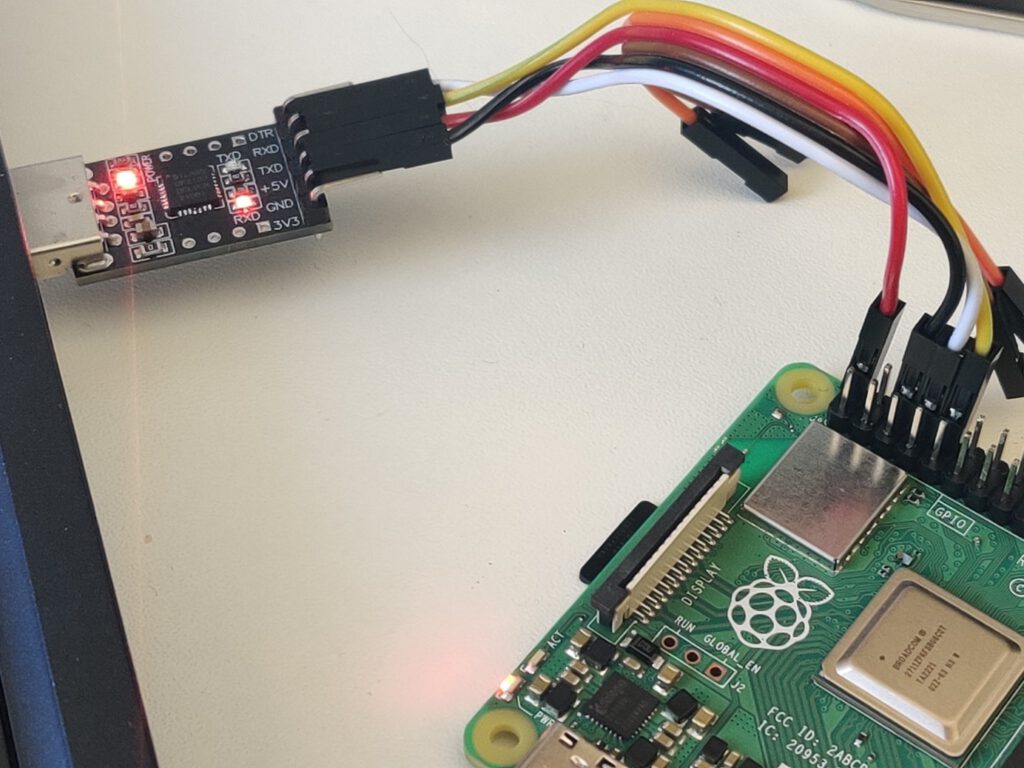
You need a USB-TTL bridge (like this one  https://www.sunrom.com/p/cp2102-usb-ttl-uart-module ) to connect the correct pins from the Raspberry to the USB. You need to connect pin 6 (ground) to the GND pin in the bridge, pin 8 (RXD) to the RXD pin of the bridge and pin 10 (TXD) to the TXD pin of the bridge. If you want to power the Raspberry via the bridge, you need to also connect pin 2 to +5V pin of the bridge. It is not recommended, because of the lower voltage, so your system might be unstable. If you don’t have a power adapter, you can simply connect a USB cable between your computer port and the USB C port of the Raspberry.  Warning! You can’t connect both a +5V connector here and a USB C power port of the Raspberry or you’ll burn the Raspberry board.

See the schema for the connection reference.

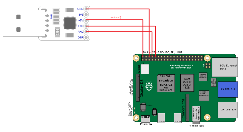
Depending on your bridge model, you may need an additional driver. I use this one:  https://www.silabs.com/developers/usb-to-uart-bridge-vcp-drivers?tab=downloads .

When you connect the +5V pin or USB-C power adapter (  again, never both at the same time! ), the Raspberry starts. Now you can open Putty and connect to your Android. Pick Serial and type COMX in the serial line definition. X is the number of your COM port. You can check it in your device manager – look for “USB to UART bridge (COM4)” or the like. The correct connection speed is 115200.

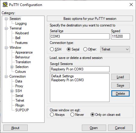
Open the connection to access the Android shell. By default, Android spawns all logs to the standard output, so you should see a lot of them right away. Anyway, it’s dual-side communication and you have full terminal access to your Android if you need to check/modify any file or call any command. Just strike enter to see the command prompt. You can even call ‘su’ to gain superuser access on your Android running on Raspberry.

Connecting via adb

If you want to use Android Debug Bridge to connect to your device, using a USB bridge is not enough. When running ‘adb devices’ on your computer, the Android Automotive OS running on Raspberry is not recognized. You can use a putty connection to turn on a TCP debug bridge instead.

Make sure you’ve connected Android and your computer to the same network. Open putty and connect to the running Android console. Log as root and enable ADB via TCP. Then check your IP address.

su
setprop service.adb.tcp.port 5555
stop adbd
start adbd
ifconfig wlan0

Now, using your Windows command line, go to the Android SDK platform-tools directory and connect to your device. As you can see, the IP address of mine Raspnberry is 192.168.50.47.

cd %userprofile%\AppData\Local\Android\Sdk\platform-tools
adb connect 192.168.50.47:5555

If you want to use ADB in WSL, you can link the Windows program in WSL using the following command.

sudo ln -s /mnt/c/Users/<your_username>/AppData/Local/Android/Sdk/platform-tools/adb.exe /usr/bin/adb

You can now use ADB to use logcat without putty or to install applications without manually transferring APK files to the SD card. Fun fact – if you use a USB bridge and USB power supply, you have two physical connections between your computer and the Android-running one, however, you still need to use ADB over WiFi to use the debug bridge.

Summary: Android Automotive OS on Raspberry Pi 4B

That’s all. Android Automotive OS 11 is running. You can install the apps you need, take them to your car, or do whatever you’d like with them.  Using hardware instead of an emulator allows you to manually manage partitions (e.g. for the  OTA update ) and connect external devices like a real GPS receiver or accelerometer. The bare metal hardware overperforms the emulator too. And most importantly – you can easily take it to your car, receive power from an in-car USB port, connect it to an ODB-II port and run real-life tests without a laptop.

 Is your project ready? Great, now you can     try doing the same with AAOS 13    .